从本篇文章开始,作者正式开始研究Python深度学习、神经网络及人工智能相关知识。前两篇文章讲解了神经网络基础概念、Theano库的安装过程及基础用法、theano实现回归神经网络,这篇文章主要讲解机器学习的基础知识,再通过theano实现分类神经网络,主要是学习"莫烦大神" 网易云视频的在线笔记,后面随着深入会讲解具体的项目及应用。基础性文章,希望对您有所帮助,也建议大家一步步跟着学习,同时文章中存在错误或不足之处,还请海涵~
"莫烦大神" 网易云视频地址:http://study.163.com/provider/1111519/course.html
从2014年开始,作者主要写了三个Python系列文章,分别是基础知识、网络爬虫和数据分析。
- Python基础知识系列:Pythonj基础知识学习与提升
- Python网络爬虫系列:Python爬虫之Selenium+Phantomjs+CasperJS
- Python数据分析系列:知识图谱、web数据挖掘及NLP


前文参考:
[Python人工智能] 一.神经网络入门及theano基础代码讲解
[Python人工智能] 二.theano实现回归神经网络分析
一.机器学习基础
首先第一部分也是莫烦老师的在线学习笔记,个人感觉挺好的基础知识,推荐给大家学习。对机器学习进行分类,包括:
1.监督学习:通过数据和标签进行学习,比如从海量图片中学习模型来判断是狗还是猫,包括分类、回归、神经网络等算法;


4.强化学习:常用于规划机器人行为准则,把计算机置于陌生环境去完成一项未知任务,比如投篮,它会自己总结失败经验和投篮命中的经验,进而惩罚或奖励机器人从而提升命中率,比如阿尔法狗;


二.神经网络基础
神经网络也称为人工神经网络ANN(Artifical Neural Network),是80年代非常流行的机器学习算法,在90年代衰退,现在随着"深度学习"和"人工智能"之势重新归来,成为最强大的机器学习算法之一。
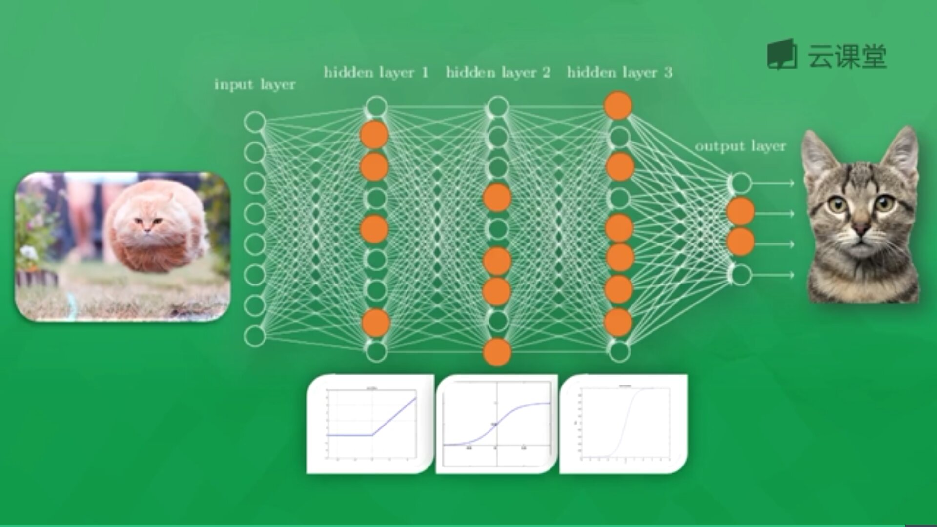
神经网络是模拟生物神经网络结构和功能的计算模型,由很多神经层组成,每一层存在着很多神经元,这些神经元是识别事物的关键。神经网络通过这些神经元进行计算学习,每个神经元有相关的激励函数(sigmoid、Softmax、tanh等),包括输入层、隐藏层(可多层或无)和输出层,当神经元计算结果大于某个阈值时会产生积极作用(输出1),相反产生抑制作用(输出0),常见的类型包括回归神经网络(画线拟合一堆散点)和分类神经网络(图像识别分类)。
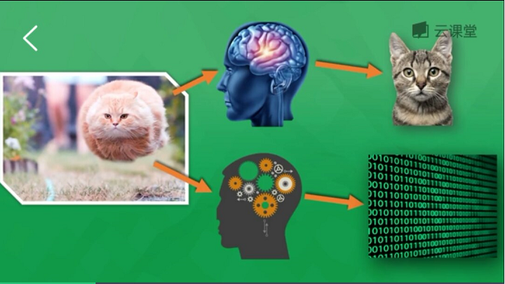
例如下面的示例,通过海量图片学习来判断一张图片是狗还是猫,通过提取图片特征转换为数学形式来判断,如果判断是狗则会反向传递这些错误信息(预测值与真实值差值)回神经网络,并修改神经元权重,通过反复学习来优化识别。
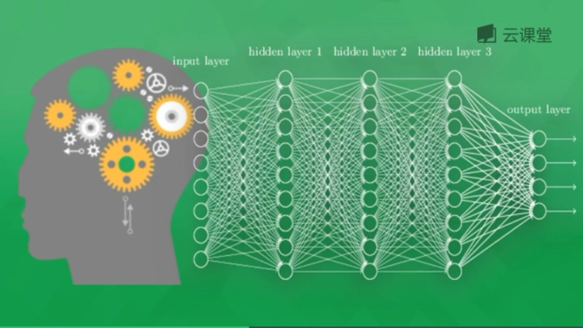
下面简单讲解"莫烦大神"网易云课程的一个示例。假设存在千万张图片,现在需要通过神经网络识别出某一张图片是狗还是猫,如下图所示共包括输入层、隐藏层(3层)和输出层。

每一个神经元都有一个激励函数,被激励的神经元传递的信息最有价值,它也决定最后的输出结果,经过海量数据的训练,最终神经网络将可以用于识别猫或狗。
三. theano实现分类神经网络
下面讲解分类神经网络的实现:
1.定义函数计算正确率
正确率为预测正确的数目占真实样本数的百分比,代码如下:
#coding:utf-8
#参考:http://study.163.com/course/courseLearn.htm?courseId=1003215006
import numpy as np
import theano.tensor as T
import theano
from theano import function

#正确率函数:预测正确数占真实值数的百分比
def computer_accuracy(y_target, y_predict):
    correct_prediction = np.equal(y_predict, y_target)
    accuracy = np.sum(correct_prediction)/len(correct_prediction)
    return accuracy
2.随机生成数据
训练样本为N,400个样本;输入特征数为feats,784个特征;随机生成数据,D = (input_values, target_class),包括输入数据和类标,其中:
(1) rng.randn(N, feats)生成400行,每行784个特征的标注正态分布数据;
(2) rng.randint(size=N, low=0, high=2)随机生成两个类别比如0和1,0代表一个类,1代表另一个类,比如猫和狗。
然后进行训练,神经网络辨别哪些是狗哪些是对应的猫。接下来编辑神经网络,用D放到图片中进行训练。
#coding:utf-8
import numpy as np
import theano.tensor as T
import theano
from theano import function
#定义分类:预测正确数占真实值数的百分比
def computer_accuracy(y_target, y_predict):
correct_prediction = np.equal(y_predict, y_target)
accuracy = np.sum(correct_prediction)/len(correct_prediction)
return accuracy
#生成虚拟的data
rng = np.random
#训练数量:400个学习样本
N = 400
#输入特征数
feats = 784
#generate a datasets: D = (input_values, target_class)
D = (rng.randn(N, feats), rng.randint(size=N, low=0, high=2))
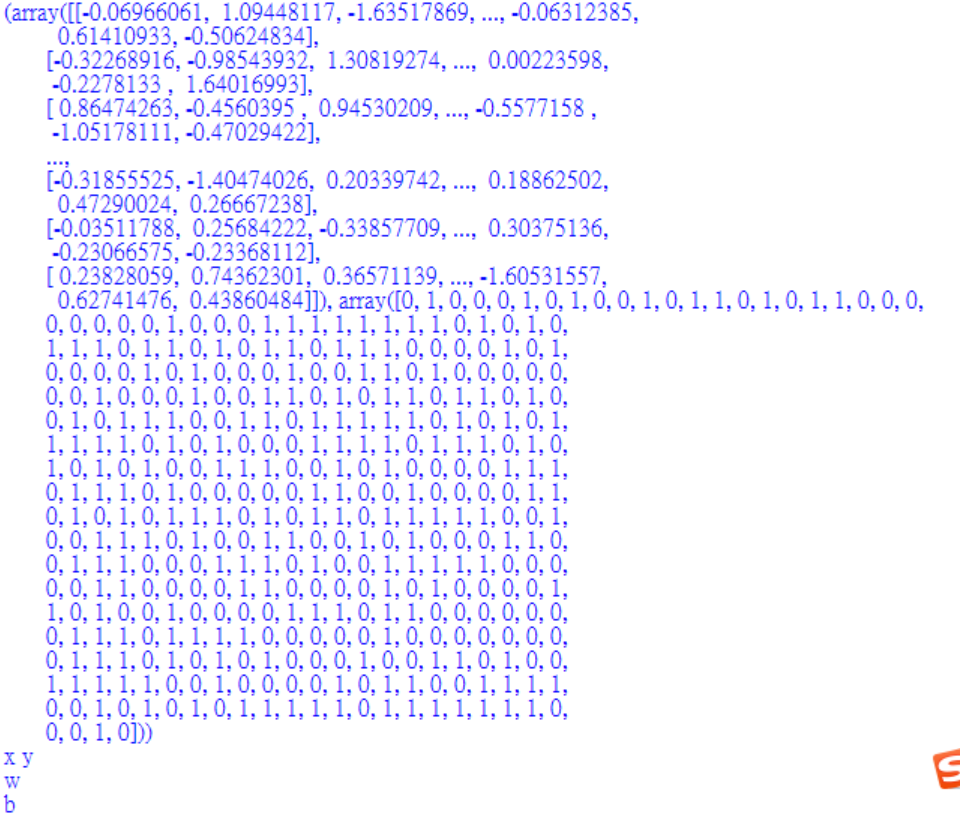
print(D)
输出的数据如下图所示:
(array([[-1.03486767,  0.09141203, -2.14011897, ...,  0.24325359,
        -1.07465997,  0.74784503],
       [ 1.09143969,  1.5014381 , -0.12580536, ..., -1.63516987,
         0.51615268,  1.51542425],
       [ 1.26905541, -0.54147591, -0.23159387, ...,  0.22647348,
        -0.93035893,  1.19128709],
       ...,
       [-0.53222844,  0.05877263, -1.05092742, ..., -1.07296129,
         1.11237909,  0.86891936],
       [-2.91024609,  0.09091794, -2.34392907, ..., -1.09686952,
         1.08838878,  0.79766499],
       [ 0.12949081, -0.0893665 , -0.43766707, ..., -0.66029383,
         0.03997112,  1.05149843]]),
array([1, 0, 0, 0, 0, 1, 1, 1, 0, 0, 0, 1, 0, 1, 1, 1, 0, 0, 1, 0, 1, 1,
       1, 1, 0, 1, 1, 1, 0, 1, 0, 0, 0, 1, 1, 1, 0, 0, 0, 0, 1, 0, 1, 1,
       1, 1, 0, 1, 0, 1, 0, 0, 0, 0, 1, 0, 1, 0, 1, 1, 0, 0, 1, 1, 0, 0,
       0, 0, 1, 0, 0, 1, 1, 0, 0, 1, 0, 1, 0, 1, 0, 0, 1, 1, 1, 1, 0, 1,
       1, 0, 1, 1, 1, 0, 0, 0, 0, 1, 0, 0, 0, 1, 0, 0, 1, 0, 1, 0, 1, 1,
       0, 0, 0, 1, 1, 1, 1, 1, 0, 0, 1, 0, 0, 0, 1, 1, 0, 1, 0, 0, 0, 1,
       0, 1, 0, 0, 1, 1, 1, 0, 1, 1, 0, 0, 0, 1, 0, 0, 1, 0, 0, 1, 0, 0,
       1, 1, 0, 0, 1, 1, 1, 0, 0, 1, 0, 1, 0, 1, 1, 0, 0, 1, 0, 0, 1, 1,
       1, 0, 0, 1, 1, 1, 0, 1, 1, 0, 0, 0, 1, 1, 1, 1, 1, 0, 0, 1, 1, 1,
       0, 0, 1, 0, 1, 1, 1, 0, 0, 1, 1, 1, 1, 0, 0, 1, 1, 1, 0, 1, 0, 0,
       0, 1, 1, 1, 1, 1, 1, 1, 0, 1, 0, 1, 0, 1, 0, 1, 0, 1, 0, 1, 1, 1,
       1, 0, 0, 1, 0, 1, 0, 1, 0, 0, 1, 0, 0, 0, 0, 0, 0, 0, 1, 0, 1, 0,
       0, 1, 0, 0, 1, 0, 1, 0, 0, 0, 1, 0, 0, 0, 0, 0, 0, 1, 1, 0, 0, 0,
       1, 1, 1, 1, 1, 1, 1, 0, 0, 1, 0, 0, 0, 0, 0, 1, 1, 0, 0, 1, 0, 1,
       0, 0, 0, 0, 1, 1, 1, 0, 0, 0, 1, 1, 1, 1, 0, 0, 0, 0, 0, 0, 1, 1,
       1, 0, 0, 0, 0, 1, 0, 1, 0, 0, 1, 0, 1, 1, 1, 0, 1, 1, 0, 1, 0, 1,
       0, 1, 1, 0, 0, 0, 0, 1, 0, 0, 1, 1, 0, 0, 1, 0, 1, 1, 1, 0, 0, 1,
       1, 1, 0, 0, 1, 0, 1, 1, 1, 1, 1, 1, 0, 1, 1, 1, 0, 1, 0, 1, 0, 0,
       0, 1, 0, 1]))
3.定义变量和初始化权重
定义Theano变量,其中x为T.dmatrix类型,y因为输出只是一个类型类型0或1,故使用dvector,也可以使用dmatrix。同时初始化权重和bias,这里不添加神经网络层,直接使用输入层和输出层,读者可以结合上节课程自己定义。
#coding:utf-8
import numpy as np
import theano.tensor as T
import theano
from theano import function

#定义分类:预测正确数占真实值数的百分比
def computer_accuracy(y_target, y_predict):
    correct_prediction = np.equal(y_predict, y_target)
    accuracy = np.sum(correct_prediction)/len(correct_prediction)
    return accuracy

#生成虚拟的data
rng = np.random

#训练数量:400个学习样本
N = 400
#输入特征数
feats = 784
#generate a datasets: D = (input_values, target_class)
#target_class: 随机分成两个类别,随机生成0和1
D = (rng.randn(N, feats), rng.randint(size=N, low=0, high=2))
print(D)


#Declare Theano symbolic variables
x = T.dmatrix('x')
y = T.dvector('y')
print(x,y)

#initialize the weights and bias
#初始化权重和bias
W = theano.shared(rng.randn(feats), name='w') #生成feats个的随机权重W,并且给个名字w
b =  theano.shared(0.1, name='b')
print(W)
print(b)
输出结果如下图所示:
4.定义计算误差
p_1 = T.nnet.sigmoid(T.dot(x,W) + b)
sigmoid激励函数(activation function)用来求概率的,如果输入的数越小,概率越接近0,输入越大,概率越接近1。这里将x与W乘积加b(T.dot(x,W) + b)放到激励函数中去。
prediction = p_1 > 0.5
定义预测值,当值大于0.5时让它等于True。
xent = -y*T.log(p_1)-(1-y)*T.log(1-p_1)
定义Cross-entropy loss function,它可以理解为cost误差,前面cost使用是平方差和,这里使用的是上述公式。
cost = xent.mean() + 0.01 * (W**2).sum()
由于xent是针对每一个样本的cost,需要求平均值变成单独的一个cost,对于整批数据的cost,故cost = xent.mean()求平均值。同时,为了克服Overfitted,在计算cost时增加 一个值(下节课补充),即0.01 * (W**2).sum()。
gW, gb = T.grad(cost, [W,b])
计算cost的梯度,这里理解为整个窗口的小控件。
#coding:utf-8
import numpy as np
import theano.tensor as T
import theano
from theano import function

#定义分类:预测正确数占真实值数的百分比
def computer_accuracy(y_target, y_predict):
    correct_prediction = np.equal(y_predict, y_target)
    accuracy = np.sum(correct_prediction)/len(correct_prediction)
    return accuracy

#生成虚拟的data
rng = np.random

#训练数量:400个学习样本
N = 400
#输入特征数
feats = 784
#generate a datasets: D = (input_values, target_class)
#target_class: 随机分成两个类别,随机生成0和1
D = (rng.randn(N, feats), rng.randint(size=N, low=0, high=2))
print(D)


#Declare Theano symbolic variables
x = T.dmatrix('x')
y = T.dvector('y')
print(x,y)

#initialize the weights and bias
#初始化权重和bias
W = theano.shared(rng.randn(feats), name='w') #生成feats个的随机权重W,并且给个名字w
b =  theano.shared(0.1, name='b')
print(W)
print(b)


#Construct Theano expression graph
#定义计算误差,激励函数sigmoid: 如果输入的数越小,概率越接近0,输入越大,概率越接近1
p_1 = T.nnet.sigmoid(T.dot(x,W) + b)
print(p_1)
#输入的数是神经网络加工后的值T.dot(x,W) + b), 然后再将这个放到激励函数中去

#大于0.1的值让它等于True
prediction = p_1 > 0.5

#梯度下降,可以理解为cost(误差)
#Cross-entropy loss function
xent = -y*T.log(p_1)-(1-y)*T.log(1-p_1)
print(xent)

cost = xent.mean() #平均值
#The cost to minimize
cost = xent.mean()  + 0.01 * (W**2).sum() #l2:为了克服Overfitted,在计算cost时加上值
print(cost)

#Compute the gradient of the cost
gW, gb = T.grad(cost, [W,b])
print(gW,gb)
输出值如下:p_1 => sigmoid.0
xent => Elemwise{sub,no_inplace}.0
cost => Elemwise{add,no_inplace}.0
gW,gb => Elemwise{add,no_inplace}.0 InplaceDimShuffle{}.0
5.编辑函数和编译模型
调用theano.function函数编译模型,两个输出即预测值和xent平均值,然后更新权重和bias,将学习的W-learning_rate*gW更新为W和b。同时,定义预测值。
#coding:utf-8
import numpy as np
import theano.tensor as T
import theano
from theano import function

#定义分类:预测正确数占真实值数的百分比
def computer_accuracy(y_target, y_predict):
    correct_prediction = np.equal(y_predict, y_target)
    accuracy = np.sum(correct_prediction)/len(correct_prediction)
    return accuracy

#生成虚拟的data
rng = np.random

#训练数量:400个学习样本
N = 400
#输入特征数
feats = 784
#generate a datasets: D = (input_values, target_class)
#target_class: 随机分成两个类别,随机生成0和1
D = (rng.randn(N, feats), rng.randint(size=N, low=0, high=2))
print(D)


#Declare Theano symbolic variables
x = T.dmatrix('x')
y = T.dvector('y')
print(x,y)

#initialize the weights and bias
#初始化权重和bias
W = theano.shared(rng.randn(feats), name='w') #生成feats个的随机权重W,并且给个名字w
b =  theano.shared(0.1, name='b')
print(W)
print(b)


#Construct Theano expression graph
#定义计算误差,激励函数sigmoid: 如果输入的数越小,概率越接近0,输入越大,概率越接近1
p_1 = T.nnet.sigmoid(T.dot(x,W) + b)
print(p_1)
#输入的数是神经网络加工后的值T.dot(x,W) + b), 然后再将这个放到激励函数中去

#大于0.1的值让它等于True
prediction = p_1 > 0.5

#梯度下降,可以理解为cost(误差)
#Cross-entropy loss function
xent = -y*T.log(p_1)-(1-y)*T.log(1-p_1)
print(xent)

cost = xent.mean() #平均值
#The cost to minimize
cost = xent.mean()  + 0.01 * (W**2).sum() #l2:为了克服Overfitted,在计算cost时加上值
print(cost)

#Compute the gradient of the cost
gW, gb = T.grad(cost, [W,b])
print(gW,gb)


#compile
#编辑函数
learning_rate = 0.1 #学习率
train = theano.function(
    inputs=[x,y],
    outputs=[prediction, xent.mean()],
    updates=((W, W-learning_rate*gW),
             (b, b-learning_rate*gb))
    ) #两个输出,更新两个数据

#定义预测 预测值为x
predict = theano.function(inputs=[x], outputs=prediction)
6.训练和预测接下来通过for循环输出结果,其中调用train(D[0],D[1])进行训练。
D[0]:D = (input_values, target_class)的第一个值,即输入变量;
D[1]:D = (input_values, target_class)的第二个值,即类标;
然后每隔50步输出结果,并查看预测正确率,函数如下:
computer_accuracy(D[1], predict(D[0]))
其中D[1]为真实的类标值,predict(D[0])是对数据预测的类标值,并计算正确率,最后输出结果。
#coding:utf-8
import numpy as np
import theano.tensor as T
import theano
from theano import function

#定义分类:预测正确数占真实值数的百分比
def computer_accuracy(y_target, y_predict):
    correct_prediction = np.equal(y_predict, y_target)
    accuracy = np.sum(correct_prediction)/len(correct_prediction)
    return accuracy

#生成虚拟的data
rng = np.random

#训练数量:400个学习样本
N = 400
#输入特征数
feats = 784
#generate a datasets: D = (input_values, target_class)
#target_class: 随机分成两个类别,随机生成0和1
D = (rng.randn(N, feats), rng.randint(size=N, low=0, high=2))
print(D)


#Declare Theano symbolic variables
x = T.dmatrix('x')
y = T.dvector('y')
print(x,y)

#initialize the weights and bias
#初始化权重和bias
W = theano.shared(rng.randn(feats), name='w') #生成feats个的随机权重W,并且给个名字w
b =  theano.shared(0.1, name='b')
print(W)
print(b)


#Construct Theano expression graph
#定义计算误差,激励函数sigmoid: 如果输入的数越小,概率越接近0,输入越大,概率越接近1
p_1 = T.nnet.sigmoid(T.dot(x,W) + b)
print(p_1)
#输入的数是神经网络加工后的值T.dot(x,W) + b), 然后再将这个放到激励函数中去

#大于0.1的值让它等于True
prediction = p_1 > 0.5

#梯度下降,可以理解为cost(误差)
#Cross-entropy loss function
xent = -y*T.log(p_1)-(1-y)*T.log(1-p_1)
print(xent)

cost = xent.mean() #平均值
#The cost to minimize
cost = xent.mean()  + 0.01 * (W**2).sum() #l2:为了克服Overfitted,在计算cost时加上值
print(cost)

#Compute the gradient of the cost
gW, gb = T.grad(cost, [W,b])
print(gW,gb)


#compile
#编辑函数
learning_rate = 0.1 #学习率
train = theano.function(
    inputs=[x,y],
    outputs=[prediction, xent.mean()],
    updates=((W, W-learning_rate*gW),
             (b, b-learning_rate*gb))
    ) #两个输出,更新两个数据

#定义预测 预测值为x
predict = theano.function(inputs=[x], outputs=prediction)

#Training
for i in range(500):
    #输入和输入标签 D = (input_values, target_class)
    pred, err = train(D[0],D[1])
    if i % 50 == 0:
        #每50步输出结果,查看多少预测正确
        print('cost:', err)
        #计算正确性 computer_accuracy(y_target, y_predict)
        print('accuracy:', computer_accuracy(D[1], predict(D[0])))


#对比两个结果,看预测是否正确
print("target values for D:")
print(D[1])
print("prediction on D:")
print(predict(D[0]))
输出结果如下所示,可以看到误差在不断减小,其预测正确率也是不断增加,最后到100%。
cost: 9.907479693928224
accuracy: 0.505
cost: 4.954027420378552
accuracy: 0.6525
cost: 2.1977148473835193
accuracy: 0.75
cost: 0.9396763739879143
accuracy: 0.875
cost: 0.40360223854133126
accuracy: 0.9575
cost: 0.17876663279172963
accuracy: 0.9825
cost: 0.0822797979378536
accuracy: 0.9925
cost: 0.048794195343816946
accuracy: 1.0
cost: 0.04187510776189411
accuracy: 1.0
cost: 0.03908366728475624
accuracy: 1.0

总结:
1.theano构建神经网络一般需要经历以下步骤:
(1) 预处理数据
generate a dataset: D = (input_values, target_class)
(2) 定义变量
Declare Theano symbolic variables
(3) 构建模型
Construct Theano expression graph
(4) 编译模型
theano.function()
train = theano.function(inputs=[x,y],outputs=[],updates=((W, W-learning_rate*gW))
predict = theano.function(inputs=[x], outputs=prediction)
(5) 训练模型
train(D[0],D[1])
(6) 预测新数据
print(predict(D[0]))
2.分类神经网络不同于回归神经网络(前一篇文章)之处:
(1) 激励函数为T.nnet.sigmoid(T.dot(x,W) + b),会用到求概率的激励函数;
(2) 它计算cost规则不同于前面平方差误差的方法,它用的是xent = -y*T.log(p_1)-(1-y)*T.log(1-p_1)。
推荐资料:
https://blog.csdn.net/zm714981790/article/details/51251759(鸢尾花分类——神经网络详解)