Programming Exercise 3:Multi-class Classification and Neural Networks
Python版本3.6
编译环境:anaconda Jupyter Notebook
链接:实验数据和实验指导书
提取码:i7co
本章课程笔记部分见:神经网络:表述(Neural Networks: Representation) 神经网络的学习(Neural Networks: Learning)
本次练习中,我们将使用逻辑回归来识别手写数字(0到9)。 我们将扩展我们在练习2中写的逻辑回归的实现,并将其应用于一对一的分类。
%matplotlib inline
#IPython的内置magic函数,可以省掉plt.show(),在其他IDE中是不会支持的
import numpy as np
import pandas as pd
import matplotlib as mpl
import matplotlib.pyplot as plt
import seaborn as sns
sns.set(style="whitegrid",color_codes=True)
import scipy.io as sio
import scipy.optimize as opt
from sklearn.metrics import classification_report#这个包是评价报告
加载数据集和可视化
它是在MATLAB的本机格式,所以要加载它在Python,我们需要使用一个SciPy工具。
data = sio.loadmat('ex3data1.mat')
X = data.get('X')
y = data.get('y')
y = y.reshape(y.shape[0])  # make it back to column vector
data
{'__header__': b'MATLAB 5.0 MAT-file, Platform: GLNXA64, Created on: Sun Oct 16 13:09:09 2011',
 '__version__': '1.0',
 '__globals__': [],
 'X': array([[0., 0., 0., ..., 0., 0., 0.],
        [0., 0., 0., ..., 0., 0., 0.],
        [0., 0., 0., ..., 0., 0., 0.],
        ...,
        [0., 0., 0., ..., 0., 0., 0.],
        [0., 0., 0., ..., 0., 0., 0.],
        [0., 0., 0., ..., 0., 0., 0.]]),
 'y': array([[10],
        [10],
        [10],
        ...,
        [ 9],
        [ 9],
        [ 9]], dtype=uint8)}
print(X.shape,y.shape)
(5000, 400) (5000,)
图像在martix X中表示为400维向量(其中有5,000个)。 400维“特征”是原始20 x 20图像中每个像素的灰度强度。类标签在向量y中作为表示图像中数字的数字类。
def plot_an_image(image):
#     """
#     image : (400,)
#     """
    fig, ax = plt.subplots(figsize=(1, 1))
    ax.matshow(image.reshape((20, 20)), cmap=mpl.cm.binary)
    plt.xticks(np.array([]))  # just get rid of ticks
    plt.yticks(np.array([]))
#绘图函数
pick_one = np.random.randint(0, 5000)
plot_an_image(X[pick_one, :])
plt.show()
print('this should be {}'.format(y[pick_one]))

this should be 5
def plot_100_image(X):
    """ sample 100 image and show them
    assume the image is square

    X : (5000, 400)
    """
    size = int(np.sqrt(X.shape[1]))

    # sample 100 image, reshape, reorg it
    sample_idx = np.random.choice(np.arange(X.shape[0]), 100)  # 100*400
    sample_images = X[sample_idx, :]

    fig, ax_array = plt.subplots(nrows=10, ncols=10, sharey=True, sharex=True, figsize=(8, 8))

    for r in range(10):
        for c in range(10):
            ax_array[r, c].matshow(sample_images[10 * r + c].reshape((size, size)),
                                   cmap=mpl.cm.binary)
            plt.xticks(np.array([]))
            plt.yticks(np.array([]))
            #绘图函数,画100张图片
plot_100_image(X)

数据预处理
# 同之前的练习一样,add intercept=1 for x0
X = np.insert(X, 0, values=np.ones(X.shape[0]), axis=1)#插入了第一列(全部为1)
X.shape
(5000, 401)
y
array([10, 10, 10, ..., 9, 9, 9], dtype=uint8)
# 扩展 5000*1 到 5000*10
#     比如 y=10 -> [0, 0, 0, 0, 0, 0, 0, 0, 0, 1]: ndarray
# y have 10 categories here. 1..10, they represent digit 0 as category 10 because matlab index start at 1
# I'll ditit 0, index 0 again
y_matrix = []

for k in range(1, 11):
    y_matrix.append((y == k).astype(int))

# last one is k==10, it's digit 0, bring it to the first position,最后一列k=10,都是0,把最后一列放到第一列
y_matrix = [y_matrix[-1]] + y_matrix[:-1]
y = np.array(y_matrix)

y.shape
(10, 5000)
y
array([[1, 1, 1, ..., 0, 0, 0],
       [0, 0, 0, ..., 0, 0, 0],
       [0, 0, 0, ..., 0, 0, 0],
       ...,
       [0, 0, 0, ..., 0, 0, 0],
       [0, 0, 0, ..., 0, 0, 0],
       [0, 0, 0, ..., 1, 1, 1]])
train 1 model(训练一维模型)
代价函数:
#sigmoid函数
def sigmoid(z):
    return 1 / (1 + np.exp(-z))
#代价函数
def cost(theta, X, y):
    ''' cost fn is -l(theta) for you to minimize'''
    return np.mean(-y * np.log(sigmoid(X @ theta)) - (1 - y) * np.log(1 - sigmoid(X @ theta)))
#加入正则化的代价函数
def regularized_cost(theta, X, y, l=1):
    '''you don't penalize theta_0'''
    theta_j1_to_n = theta[1:]
    regularized_term = (l / (2 * len(X))) * np.power(theta_j1_to_n, 2).sum()

    return cost(theta, X, y) + regularized_term
#梯度下降def gradient(theta, X, y):
def gradient(theta, X, y):
    '''just 1 batch gradient'''
    return (1 / len(X)) * X.T @ (sigmoid(X @ theta) - y)
#加入正则化的梯度下降
def regularized_gradient(theta, X, y, l=1):
    '''still, leave theta_0 alone'''
    theta_j1_to_n = theta[1:]
    regularized_theta = (l / len(X)) * theta_j1_to_n

    # by doing this, no offset is on theta_0
    regularized_term = np.concatenate([np.array([0]), regularized_theta])

    return gradient(theta, X, y) + regularized_term
def logistic_regression(X, y, l=1):
    """generalized logistic regression
    args:
        X: feature matrix, (m, n+1) # with incercept x0=1
        y: target vector, (m, )
        l: lambda constant for regularization

    return: trained parameters
    """
    # init theta
    theta = np.zeros(X.shape[1])

    # train it
    res = opt.minimize(fun=regularized_cost,
                       x0=theta,
                       args=(X, y, l),
                       method='TNC',
                       jac=regularized_gradient,
                       options={'disp': True})
    # get trained parameters
    final_theta = res.x

    return final_theta
def predict(x, theta):
    prob = sigmoid(x @ theta)
    return (prob >= 0.5).astype(int)
t0 = logistic_regression(X, y[0])
print(t0.shape)
y_pred = predict(X, t0)
print('Accuracy={}'.format(np.mean(y[0] == y_pred)))
(401,)
Accuracy=0.9974
train k model(训练k维模型)
k_theta = np.array([logistic_regression(X, y[k]) for k in range(10)])
print(k_theta.shape)
(10, 401)
进行预测
- think about the shape of k_theta, now you are making
- after that, you run sigmoid to get probabilities and for each row, you find the highest prob as the answer
def predict_all(X, all_theta):
    rows = X.shape[0]
    params = X.shape[1]
    num_labels = all_theta.shape[0]

    # same as before, insert ones to match the shape
    X = np.insert(X, 0, values=np.ones(rows), axis=1)

    # convert to matrices
    X = np.matrix(X)
    all_theta = np.matrix(all_theta)

    # compute the class probability for each class on each training instance
    h = sigmoid(X * all_theta.T)

    # create array of the index with the maximum probability
    h_argmax = np.argmax(h, axis=1)

    # because our array was zero-indexed we need to add one for the true label prediction
    h_argmax = h_argmax + 1

    return h_argmax
prob_matrix = sigmoid(X @ k_theta.T)
np.set_printoptions(suppress=True)
prob_matrix
array([[0.99577769, 0.        , 0.00053524, ..., 0.00006465, 0.00003907,
        0.00172229],
       [0.9983465 , 0.0000001 , 0.0000561 , ..., 0.00009675, 0.0000029 ,
        0.00008486],
       [0.99140504, 0.        , 0.0005686 , ..., 0.00000654, 0.02654245,
        0.00197582],
       ...,
       [0.00000068, 0.04140879, 0.00320814, ..., 0.0001273 , 0.00297237,
        0.70757659],
       [0.00001843, 0.00000013, 0.00000009, ..., 0.00164616, 0.0681586 ,
        0.86109922],
       [0.02879654, 0.        , 0.00012981, ..., 0.36617522, 0.0049769 ,
        0.14830126]])
y_pred = np.argmax(prob_matrix, axis=1)#返回沿轴axis最大值的索引,axis=1代表行
y_pred
array([0, 0, 0, ..., 9, 9, 7], dtype=int64)
y_answer = data['y'].copy()
y_answer[y_answer==10] = 0
print(classification_report(y_answer, y_pred))
              precision    recall  f1-score   support

           0       0.97      0.99      0.98       500
           1       0.95      0.99      0.97       500
           2       0.95      0.92      0.93       500
           3       0.95      0.91      0.93       500
           4       0.95      0.95      0.95       500
           5       0.92      0.92      0.92       500
           6       0.97      0.98      0.97       500
           7       0.95      0.95      0.95       500
           8       0.93      0.92      0.92       500
           9       0.92      0.92      0.92       500

   micro avg       0.94      0.94      0.94      5000
   macro avg       0.94      0.94      0.94      5000
weighted avg       0.94      0.94      0.94      5000
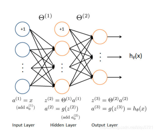
神经网络模型图示
def load_weight(path):
    data = sio.loadmat(path)
    return data['Theta1'], data['Theta2']
theta1, theta2 = load_weight('ex3weights.mat')
theta1.shape, theta2.shape
((25, 401), (10, 26))
data = sio.loadmat('ex3data1.mat')
X = data.get('X')
y = data.get('y')
y = y.reshape(y.shape[0])  # make it back to column vector
# 同之前的练习一样,add intercept=1 for x0
X = np.insert(X, 0, values=np.ones(X.shape[0]), axis=1)#插入了第一列(全部为1)
X.shape,y.shape
((5000, 401), (5000,))
feed forward prediction(前馈预测)
a1 = X
z2 = a1 @ theta1.T# (5000, 401) @ (25,401).T = (5000, 25)
z2.shape
(5000, 25)
z2 = np.insert(z2, 0, values=np.ones(z2.shape[0]), axis=1)
a2 = sigmoid(z2)
a2.shape
(5000, 26)
z3 = a2 @ theta2.T
z3.shape
(5000, 10)
a3 = sigmoid(z3)
a3.shape
(5000, 10)
y_pred = np.argmax(a3, axis=1) + 1  # numpy is 0 base index, +1 for matlab convention,返回沿轴axis最大值的索引,axis=1代表行
y_pred.shape
(5000,)
y_pred
array([10, 10, 10, ..., 9, 9, 9], dtype=int64)
准确率
虽然人工神经网络是非常强大的模型,但训练数据的准确性并不能完美预测实际数据,在这里很容易过拟合。
print(classification_report(y, y_pred))
              precision    recall  f1-score   support

           1       0.97      0.98      0.97       500
           2       0.98      0.97      0.97       500
           3       0.98      0.96      0.97       500
           4       0.97      0.97      0.97       500
           5       0.98      0.98      0.98       500
           6       0.97      0.99      0.98       500
           7       0.98      0.97      0.97       500
           8       0.98      0.98      0.98       500
           9       0.97      0.96      0.96       500
          10       0.98      0.99      0.99       500

   micro avg       0.98      0.98      0.98      5000
   macro avg       0.98      0.98      0.98      5000
weighted avg       0.98      0.98      0.98      5000