作业说明
Exercise 3,Week 4,使用Octave实现手写数字0-9的识别,采用两种方式(1)逻辑回归多分类(2)三层神经网络多分类。对比结果。
每张图片20px * 20px,也就是一共400个特征(因为Octave里从1开始。所以将0映射为10)
(1)逻辑回归多分类:实现 lrCostFunction 计算代价和梯度。实现 OneVsAll 使用 fmincg 函数进行训练。使用 OneVsAll 里训练好的 theta 对 X 的数据类型进行预测,得到平均准确率。
(2)神经网络:两层 theta 权重值在 ex3weights 里已提供。参数不需要调,只需要在 predict 里进行矩阵计算,即可得到分类结果。
数据集 :ex3data1.mat 。手写数字图片数据。5000个样例。数据集X的维度为5000 * 400
ex3weights.mat。神经网络每一层的权重。
文件清单
ex3.m - Octave/MATLAB script that steps you through part 1
ex3 nn.m - Octave/MATLAB script that steps you through part 2
ex3data1.mat - Training set of hand-written digits
ex3weights.mat - Initial weights for the neural network exercise
submit.m - Submission script that sends your solutions to our servers
displayData.m - Function to help visualize the dataset
fmincg.m - Function minimization routine (similar to fminunc)
sigmoid.m - Sigmoid function
[?] lrCostFunction.m - Logistic regression cost function
[?] oneVsAll.m - Train a one-vs-all multi-class classi er
[?] predictOneVsAll.m - Predict using a one-vs-all multi-class classi er
[?] predict.m - Neural network prediction function
* 为必须要完成的
结论
矩阵运算tricky的地方在于维度对应,哪里需要转置很关键。
逻辑回归多分类
一、在数据集X里随机选择100个数字,绘制
displayData.m:
function [h, display_array] = displayData(X, example_width)
%DISPLAYDATA Display 2D data in a nice grid
%   [h, display_array] = DISPLAYDATA(X, example_width) displays 2D data
%   stored in X in a nice grid. It returns the figure handle h and the
%   displayed array if requested.

% Set example_width automatically if not passed in
if ~exist('example_width', 'var') || isempty(example_width)
    example_width = round(sqrt(size(X, 2)));
end

% Gray Image
colormap(gray);

% Compute rows, cols
[m n] = size(X);
example_height = (n / example_width);

% Compute number of items to display
display_rows = floor(sqrt(m));
display_cols = ceil(m / display_rows);

% Between images padding
pad = 1;

% Setup blank display
display_array = - ones(pad + display_rows * (example_height + pad), ...
                       pad + display_cols * (example_width + pad));

% Copy each example into a patch on the display array
curr_ex = 1;
for j = 1:display_rows
    for i = 1:display_cols
        if curr_ex > m,
            break;
        end
        % Copy the patch

        % Get the max value of the patch
        max_val = max(abs(X(curr_ex, :)));
        display_array(pad + (j - 1) * (example_height + pad) + (1:example_height), ...
                      pad + (i - 1) * (example_width + pad) + (1:example_width)) = ...
                        reshape(X(curr_ex, :), example_height, example_width) / max_val;
        curr_ex = curr_ex + 1;
    end
    if curr_ex > m,
        break;
    end
end

% Display Image
h = imagesc(display_array, [-1 1]);

% Do not show axis
axis image off

drawnow;

end
ex3.m里的调用
load('ex3data1.mat'); % training data stored in arrays X, y
m = size(X, 1);

% Randomly select 100 data points to display
rand_indices = randperm(m);
sel = X(rand_indices(1:100), :);

displayData(sel);
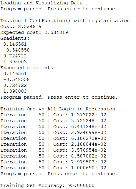
运行效果如下:

二、代价函数
注意:θ0不参与正则化。
正则化逻辑回归的代价函数如下,分为三项:
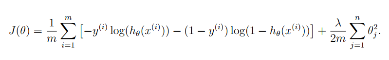
梯度下降算法如下:


lrCostFunction.m:
function [J, grad] = lrCostFunction(theta, X, y, lambda)

m = length(y); % number of training examples

temp = theta; temp(1) = 0;   % because we don't add anything for j = 0

% 第一项
part1 = -y' * log(sigmoid(X * theta));
% 第二项
part2 = (1 - y)' * log(1 - sigmoid(X * theta));

% 正则项
regTerm = lambda / 2 / m * temp' * temp;
J = 1 / m * (part1 - part2) + regTerm;

% 梯度
grad = 1 / m * X' *((sigmoid(X * theta) - y)) + lambda / m * temp;

grad = grad(:);

end
正则化之后的代价函数同时返回代价 J 和 grad 梯度。这里和上个星期实现的二分类逻辑回归代码是一样的。
三、训练oneVsAll多分类模型
week2逻辑回归分类的目标是区分两种类型。写好代价函数之后,调用一次 fminunc 函数,得到 theta、就可以画出 boundary。
但是多分类中需要训练 K 个分类器,所以多了一个 oneVsAll.m。其实就是循环 K 次,得到一个 theta矩阵(row 为 K,column为特征值个数)。
function [all_theta] = oneVsAll(X, y, num_labels, lambda)

% Some useful variables
m = size(X, 1);
n = size(X, 2);

% You need to return the following variables correctly
all_theta = zeros(num_labels, n + 1);

% Add ones to the X data matrix
X = [ones(m, 1) X];

initial_theta = zeros(n + 1, 1);

options = optimset('GradObj', 'on', 'MaxIter', 50);

% Run fmincg to obtain the optimal theta
% This function will return theta and the cost
for i = 1 : num_labels,
  [theta] = ...
    fmincg(@(t)(lrCostFunction(t, X, (y == i), lambda)), ...
         initial_theta, options);
  all_theta(i,:) = theta';
end;

end
多分类使用的 Octave 函数是 fmincg 不是 fminunc,fmincg更适合参数多的情况。
注意这里用到了 y == i,这个操作将 y 中每个数据和 i 进行比较。得到的矩阵中(这里是向量)相同的为1,不同的为0。
ex3.m 里的调用
lambda = 0.1;
[all_theta] = oneVsAll(X, y, num_labels, lambda);
四、使用OneVsAll分类器进行预测
predictOneVsAll.m
function p = predictOneVsAll(all_theta, X)

m = size(X, 1);
num_labels = size(all_theta, 1);

% You need to return the following variables correctly
p = zeros(size(X, 1), 1);

% Add ones to the X data matrix
X = [ones(m, 1) X];

temp = X * all_theta';
[x, p] = max(temp,[],2);

end
将 X 与 theta 相乘得到预测结果,得到一个 5000*10 的矩阵,每行对应一个分类结果(只有一个1,其余为0)。
题目要求返回的矩阵 p 是一个 5000*1 的矩阵。每行是 1-K 的数字。使用 max 函数,得到两个返回值。第一个 x 是一个全1的向量,没用。第二个是 1 所在的 index,也就是对应的类别。
ex3.m 中的调用:
pred = predictOneVsAll(all_theta, X);
fprintf('\nTraining Set Accuracy: %f\n', mean(double(pred == y)) * 100);
神经网络
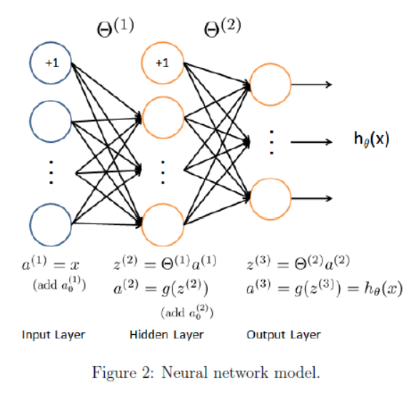
这里g(z) 使用 sigmoid 函数。
神经网络中,从上到下的每个原点是 feature 特征 x0, x1, x2...,不是实例。计算过程其实就是 feature 一层一层映射的过程。一层转换之后,feature可能变多、也可能变少。下一层 i+1层 feature 的个数是通过权重矩阵里当前 θ(i) 的 row 行数来控制。
两层权重 θ 已经在 ex3weights.mat 里给出。从a1映射到a2权重矩阵 θ1为 25 * 401,从a2映射到a3权重矩阵 θ2为10 * 26。因为最后有10个分类。(这意味着运算的时候要注意转置)
一、使用OneVsAll分类器进行预测
权重已经在文件中给出了,只需要矩阵相乘,预测就好了
predict.m :
function p = predict(Theta1, Theta2, X)
%PREDICT Predict the label of an input given a trained neural network
%   p = PREDICT(Theta1, Theta2, X) outputs the predicted label ofxgiven the
%   trained weights of a neural network (Theta1, Theta2)

% Useful values m = size(X, 1); num_labels = size(Theta2, 1); % You need to return the following variables correctly p = zeros(size(X, 1), 1); % ====================== YOUR CODE HERE ====================== % Instructions: Complete the following code to make predictions using % your learned neural network. You should set p to a % vector containing labels between 1 to num_labels. % % Hint: The max function might come in useful. In particular, the max % function can also return the index of the max element, for more % information see 'help max'. If your examples are in rows, then, you % can use max(A, [], 2) to obtain the max for each row. %0 % Add ones to thexdata matrix a1 = [ones(m, 1) X]; %5000x401 a2 = sigmoid(a1 * Theta1'); %5000x401乘以401x25得到5000x25。即把401个feature映射到25  a2 = [ones(m, 1) a2]; %5000x26 a3 = sigmoid(a2 * Theta2'); %5000x26乘以26x10得到5000x10。即把26个feature映射到10  [x,p] = max(a3,[],2);  %和上面逻辑回归多分类一样,最后使用 max 函数获得分类结果。 % ========================================================================= end
二、预测结果
em3_nn.m 里的调用
%% Setup the parameters you will use for this exercise
input_layer_size  = 400;  % 20x20 Input Images of Digits
hidden_layer_size = 25; % 25 hidden units num_labels = 10; % 10 labels, from 1 to 10 % (note that we have mapped "0" to label 10) load('ex3weights.mat'); pred = predict(Theta1, Theta2, X); fprintf('\nTraining Set Accuracy: %f\n', mean(double(pred == y)) * 100); % To give you an idea of the network's output, you can also run % through the examples one at the a time to see what it is predicting. % Randomly permute examples    随机获取数字,显示预测结果 rp = randperm(m); for i = 1:m % Display fprintf('\nDisplaying Example Image\n'); displayData(X(rp(i), :)); pred = predict(Theta1, Theta2, X(rp(i),:)); fprintf('\nNeural Network Prediction: %d (digit %d)\n', pred, mod(pred, 10)); % Pause with quit option s = input('Paused - press enter to continue, q to exit:','s'); if s == 'q' break end end
运行结果:
准确率 Training Set Accuracy: 97.520000

![]()


这里我比较疑惑的一点是。代码中没对 0 进行特殊处理,为什么能预测成10。后来一想 整个计算过程都是权重矩阵控制的,给的 weights 文件里已经是调整好的结果了,0 就是会被分类成10。
所以神经网络最主要的还是调参啊,调 θ 矩阵。
三、关于矩阵相乘
矩阵这里转置总是出问题。仔细思考一下
![]()
(1)假设只有一个实例 x,而且它像图中一样是一个列向量。那根据神经网络的公式,最相符的应该是 θ(i) * x。最后的得到的是 K 维列向量。
(2)但实际情况中,训练数据通常一行一个实例。如果严格按图和公式去计算,(θ(i) * XT)T 就需要将 X 先转置过来,最后再转置回去。应该是下面的代码,但是明显能看出比上面的方法麻烦:
a1 = [ones(1, m); X'];      %401x5000
a2 = sigmoid(Theta1 * a1);  %25x401 乘以 401x5000   得到25x5000

a2 = [ones(1, m); a2];      %26x5000
a3 = sigmoid(Theta2 * a2);  %10x26 乘以 26x5000    得到10x5000

a3 = a3'; % 5000x10
(3)所以用 X * θ(i)T 替换 (θ(i) * XT)T
a1 = [ones(m, 1) X];    %5000x401
a2 = sigmoid(a1 * Theta1');  %5000x401乘以401x25得到5000x25。即把401个feature映射到25

a2 = [ones(m, 1) a2];    %5000x26
a3 = sigmoid(a2 * Theta2');  %5000x26乘以26x10得到5000x10。即把26个feature映射到10
完整代码:https://github.com/madoubao/coursera_machine_learning/tree/master/homework/machine-learning-ex3/ex3