Part 1：Happy House 的人脸识别

本周的第一个作业我们将完成一个人脸识别系统。

人脸识别问题可以分为两类：

人脸验证: 输入图片，验证是不是A
- 1:1 识别
- 举例：人脸解锁手机，人脸刷卡
人脸识别: 有一个库，输入图片，验证是不是库里的一员
- 1:K 识别
- 举例：员工门禁

FaceNet 通过神经网络学习将图片编码为128维数字向量。通过比较两个128维向量的相似度来确定两张图片是否是同一个人。

在这个作业中，你需要：

实现三元组损失函数
使用一个预训练模型将图片转换为128维数字向量
运用这些128维的数字向量来执行人脸验证和人脸识别

在这个练习中，你将使用一个预训练模型，该模型表示图片时使用”通道在前”的维度表示，(m,nC,nH,nW) 而不是之前的 (m,nH,nW,nC)。

开源社区中两种表示方法都很常见，没有统一的标准。

导包

from keras.models import Sequential
from keras.layers import Conv2D, ZeroPadding2D, Activation, Input, concatenate
from keras.models import Model
from keras.layers.normalization import BatchNormalization
from keras.layers.pooling import MaxPooling2D, AveragePooling2D
from keras.layers.merge import Concatenate
from keras.layers.core import Lambda, Flatten, Dense
from keras.initializers import glorot_uniform
from keras.engine.topology import Layer
from keras import backend as K
K.set_image_data_format('channels_first')
import cv2
import os
import numpy as np
from numpy import genfromtxt
import pandas as pd
import tensorflow as tf
from fr_utils import *
from inception_blocks_v2 import *

%matplotlib inline
%load_ext autoreload
%autoreload 2

np.set_printoptions(threshold=np.nan)

0 朴素人脸验证

在人脸验证中，给你两张图片，你需要给出这两张图片是否是同一个人。最简单的方式是一一比较两张图片的像素，如果两张图片的像素距离小于一个阈值，就认为是同一个人。

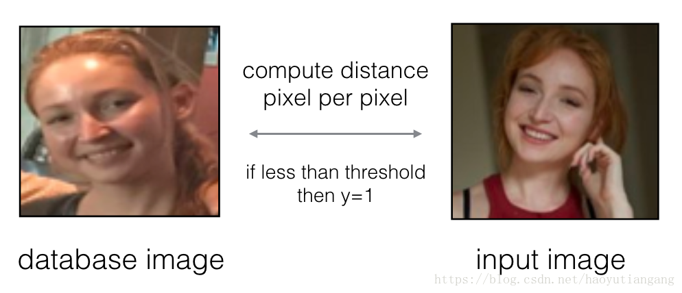
当然，这个算法的表现着实很差，因为图片的像素会随着灯光，角度，头部位置等元素而剧烈变化。

你会发现，不通过原始图片进行比较，而是通过机器学习将图片进行编码为相同维度的向量，然后计算向量的距离来识别是否是同一个人，拥有更高的准确率。

1 将图片编码为128维的向量

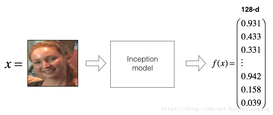
1.1 使用ConvNet编码图片

FaceNet模型需要大量的数据和时间去训练，这里我们使用别人已经训练好的模型，你也可以从inception_blocks.py看到模型是怎么实现的。

你需要知道：

输入：96x96 RGB：(m,nC,nH,nW) = (m,3,96,96)
输出： (m,128)

FRmodel = faceRecoModel(input_shape=(3, 96, 96))
print("Total Params:", FRmodel.count_params())
# Total Params: 3743280

在模型的最后一层使用128个神经元的全连接层，模型确保输出维度为128，然后就可以利用编码后的向量比较两个图片了。

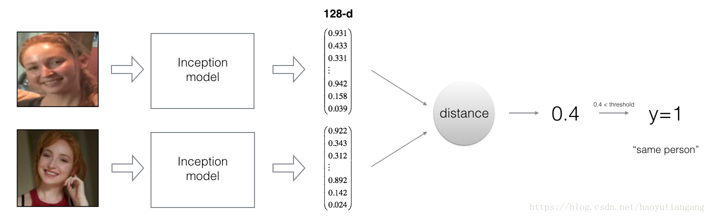
如果符合以下条件，编码方式就是好的：

同一个人的两张照片的编码非常相似
不同人的两张照片编码差别很大

三元组损失函数(triplet loss function) 很好的实现了上述要求，将同一个人的两张照片 (anchor 和 Positive) 的编码推得很近，将不同人的两张照片 (anchor 和 Negative) 的编码拉的很远。

1.2 三元组损失

对于一张图片 x，另其编码为f(x), 其中f是从神经网络计算出来的

三元组图片：(A, P, N)

A：Anchor – 一个人的图片
P：Positive – 与Ancher同一个人的图片
N：Negative – 与Ancher不同人的图片

我们训练集中已经有这些三元组数据，用(A(i), P(i), N(i)) 来表示训练集第i个样本。

你需要确保 A(i) 到 P(i) 的距离至少比到 N(i) 的距离远一个alpha。

∣ ∣ f (A^{(i)}) - f (P^{(i)}) ∣ ∣_{2}^{2} + α <∣∣ f (A^{(i)}) - f (N^{(i)}) ∣ ∣_{2}^{2}

$\mid \mid f(A^{(i)}) - f(P^{(i)}) \mid \mid_2^2 + \alpha < \mid \mid f(A^{(i)}) - f(N^{(i)}) \mid \mid_2^2$

我们将最小化如下的三元组损失 J：

z = \sum_{i = 1}^{N} [\underset{(1)}{\underset{⏟}{∣ ∣ f (A^{(i)}) - f (P^{(i)}) ∣ ∣_{2}^{2}}} - \underset{(2)}{\underset{⏟}{∣ ∣ f (A^{(i)}) - f (N^{(i)}) ∣ ∣_{2}^{2}}} + α]

$z = \sum^{N}_{i=1} \large[ \small \underbrace{\mid \mid f(A^{(i)}) - f(P^{(i)}) \mid \mid_2^2}_\text{(1)} - \underbrace{\mid \mid f(A^{(i)}) - f(N^{(i)}) \mid \mid_2^2}_\text{(2)} + \alpha \large ]$

J = m a x (z, 0)

$\mathcal{J} = max(z, 0)$
注意：

公式中(1)部分是”A”到”P”的平方距离，我们想要缩小
公式中(2)部分是”A”到”N”的平方距离，我们想要扩大，所以这里用了减法，而减完之后是个距离的负值
alpha 是一个距离阈值的超参数，需要手动设定，这里使用0.2

很多实现都是先将图片编码进行归一化再比较的，这里我们不用考虑。

练习：实现三元组损失函数

计算”A”到”P”的距离
$∣ ∣ f (A^{(i)}) - f (P^{(i)}) ∣ ∣_{2}^{2}$ $\mid \mid f(A^{(i)}) - f(P^{(i)}) \mid \mid_2^2$
计算”A”到”N”的距离
$∣ ∣ f (A^{(i)}) - f (N^{(i)}) ∣ ∣_{2}^{2}$ $\mid \mid f(A^{(i)}) - f(N^{(i)}) \mid \mid_2^2$
计算 z
$z =∣∣ f (A^{(i)}) - f (P^{(i)}) ∣ - ∣∣ f (A^{(i)}) - f (N^{(i)}) ∣ ∣_{2}^{2} + α$ $z = \mid \mid f(A^{(i)}) - f(P^{(i)}) \mid - \mid \mid f(A^{(i)}) - f(N^{(i)}) \mid \mid_2^2 + \alpha$
计算 z 与 0 的最大值
$J = m a x (z, 0)$ $\mathcal{J} = max(z, 0)$

有用的函数：tf.reduce_sum(), tf.square(), tf.subtract(), tf.add(), tf.maximum()

# GRADED FUNCTION: triplet_loss

def triplet_loss(y_true, y_pred, alpha = 0.2):
    """
    Implementation of the triplet loss as defined by formula (3)

    Arguments:
    y_true -- true labels, required when you define a loss in Keras, you don't need it in this function.
    y_pred -- python list containing three objects:
            anchor -- the encodings for the anchor images, of shape (None, 128)
            positive -- the encodings for the positive images, of shape (None, 128)
            negative -- the encodings for the negative images, of shape (None, 128)

    Returns:
    loss -- real number, value of the loss
    """

    anchor, positive, negative = y_pred[0], y_pred[1], y_pred[2]

    ### START CODE HERE ### (≈ 4 lines)
    # Step 1: Compute the (encoding) distance between the anchor and the positive, you will need to sum over axis=-1
    pos_dist = tf.reduce_sum(tf.square(tf.subtract(anchor, positive)))
    # Step 2: Compute the (encoding) distance between the anchor and the negative, you will need to sum over axis=-1
    neg_dist = tf.reduce_sum(tf.square(tf.subtract(anchor, negative)))
    # Step 3: subtract the two previous distances and add alpha.
    basic_loss = tf.add(tf.subtract(pos_dist,neg_dist), alpha)
    # Step 4: Take the maximum of basic_loss and 0.0. Sum over the training examples.
    loss = tf.reduce_sum(tf.maximum(basic_loss, 0.))
    ### END CODE HERE ###

    return loss

#########################################################

with tf.Session() as test:
    tf.set_random_seed(1)
    y_true = (None, None, None)
    y_pred = (tf.random_normal([3, 128], mean=6, stddev=0.1, seed = 1),
              tf.random_normal([3, 128], mean=1, stddev=1, seed = 1),
              tf.random_normal([3, 128], mean=3, stddev=4, seed = 1))
    loss = triplet_loss(y_true, y_pred)

    print("loss = " + str(loss.eval()))

# loss = 350.026

2 导入预训练模型

FaceNet已经使用最小化三元组损失训练过了，但是训练需要大量的数据和时间，这里我们使用训练好的模型。

FRmodel.compile(optimizer = 'adam', loss = triplet_loss, metrics = ['accuracy'])
load_weights_from_FaceNet(FRmodel)

三组个人图片的编码和距离示例

现在我们用这个模型来进行人脸验证和人脸识别。

3 应用模型

回到Happy House! 因为你在之前的作业中设计了快乐识别模型，成员们幸福快乐的住在Happy House里。

然而，还是出现了一些问题：由于Happy House 特别Happy,很多邻居都来串门，使房间变得很拥挤，对大家产生了负面的影响。这些随机进来的快乐的人还吃光了你们所有的食物。

所以，你决定改变门禁策略，不再让快乐的人随便进来，而是采用一个人脸验证系统来保证只有名单上的人可以进来，给每个乘客发一张ID卡，每个进来的人都必须刷卡，人脸验证系统来验证刷卡的人是不是本人。

3.1 人脸验证

让我们建立一个访客照片的编码向量数据集, 使用 img_to_encoding(image_path, model) 方法将图片转换为128维的向量。

database = {}
database["danielle"] = img_to_encoding("images/danielle.png", FRmodel)
database["younes"] = img_to_encoding("images/younes.jpg", FRmodel)
database["tian"] = img_to_encoding("images/tian.jpg", FRmodel)
database["andrew"] = img_to_encoding("images/andrew.jpg", FRmodel)
database["kian"] = img_to_encoding("images/kian.jpg", FRmodel)
database["dan"] = img_to_encoding("images/dan.jpg", FRmodel)
database["sebastiano"] = img_to_encoding("images/sebastiano.jpg", FRmodel)
database["bertrand"] = img_to_encoding("images/bertrand.jpg", FRmodel)
database["kevin"] = img_to_encoding("images/kevin.jpg", FRmodel)
database["felix"] = img_to_encoding("images/felix.jpg", FRmodel)
database["benoit"] = img_to_encoding("images/benoit.jpg", FRmodel)
database["arnaud"] = img_to_encoding("images/arnaud.jpg", FRmodel)

现在你就可以验证刷卡的是不是本人了。

练习: 实现 verify() 方法

计算门前人照片的编码向量
计算ID所有者编码向量与门前照片向量的距离
如果距离小于0.7 就开门，否则不开门

这里我们是有L2距离：np.linalg.norm，而不是L2距离的平方
门槛阈值为 0.7

# GRADED FUNCTION: verify

def verify(image_path, identity, database, model):
    """
    Function that verifies if the person on the "image_path" image is "identity".

    Arguments:
    image_path -- path to an image
    identity -- string, name of the person you'd like to verify the identity. Has to be a resident of the Happy house.
    database -- python dictionary mapping names of allowed people's names (strings) to their encodings (vectors).
    model -- your Inception model instance in Keras

    Returns:
    dist -- distance between the image_path and the image of "identity" in the database.
    door_open -- True, if the door should open. False otherwise.
    """

    ### START CODE HERE ###

    # Step 1: Compute the encoding for the image. Use img_to_encoding() see example above. (≈ 1 line)
    encoding = img_to_encoding(image_path, model)

    # Step 2: Compute distance with identity's image (≈ 1 line)
    dist = np.linalg.norm(encoding - database[identity])

    # Step 3: Open the door if dist < 0.7, else don't open (≈ 3 lines)
    if dist < 0.7:
        print("It's " + str(identity) + ", welcome home!")
        door_open = True
    else:
        print("It's not " + str(identity) + ", please go away")
        door_open = False

    ### END CODE HERE ###

    return dist, door_open

Younes 想进来，然后门上摄像头拍了一张图片(“images/camera_0.jpg”), 然我们验证一下吧。

verify("images/camera_0.jpg", "younes", database, FRmodel)

# It's younes, welcome home!
# 
# (0.65939283, True)

Benoit 上周打破了鱼缸，已经被赶出去了，数据库也除名了，他拿了 Kian 的ID卡想进来试图说自己就是Kian, 门上摄像头采集看他一张照片(“images/camera_2.jpg”), 让我们验证一下吧。

verify("images/camera_2.jpg", "kian", database, FRmodel)

#It's not kian, please go away
#
#(0.86224014, False)

3.2 人脸识别

你的人脸验证系统通常工作的很好，但是自从Kian的ID卡被偷了，晚上他回来后都进不来了。

为了减少这种乌龙的发生，你想将你的人脸验证系统改造成人脸识别系统。这样大家就不用带卡了，但有权限的人走到门前，门将会自动为他解锁。

为了实现人脸识别系统，你需要输入一张图片，然后系统识别这个人在不在有权限人员集合中。和之前的人脸验证系统不一样，这次你不再需要输入某人的姓名或ID了。

练习：实现 who_is_it()

计算门前人照片的编码向量
从数据库找出与门前人编码向量距离最小的编码向量。
- 初始化最小距离(min_dist)为一个足够大的值(100)。用来跟踪距离最小值。
- 循环数据库中的人的编码向量：for (name, db_enc) in database.items()
- 计算门前向量和当前循环向量的L2距离
- 如果当前距离小于最小距离(min_dist)，更新最小距离，记录当前循环变量的人的名字

# GRADED FUNCTION: who_is_it

def who_is_it(image_path, database, model):
    """
    Implements face recognition for the happy house by finding who is the person on the image_path image.

    Arguments:
    image_path -- path to an image
    database -- database containing image encodings along with the name of the person on the image
    model -- your Inception model instance in Keras

    Returns:
    min_dist -- the minimum distance between image_path encoding and the encodings from the database
    identity -- string, the name prediction for the person on image_path
    """

    ### START CODE HERE ### 

    ## Step 1: Compute the target "encoding" for the image. Use img_to_encoding() see example above. ## (≈ 1 line)
    encoding = img_to_encoding(image_path, model)

    ## Step 2: Find the closest encoding ##

    # Initialize "min_dist" to a large value, say 100 (≈1 line)
    min_dist = 100

    # Loop over the database dictionary's names and encodings.
    for (name, db_enc) in database.items():

        # Compute L2 distance between the target "encoding" and the current "emb" from the database. (≈ 1 line)
        dist = np.linalg.norm(encoding - db_enc)

        # If this distance is less than the min_dist, then set min_dist to dist, and identity to name. (≈ 3 lines)
        if dist < min_dist:
            min_dist = dist
            identity = name

    ### END CODE HERE ###

    if min_dist > 0.7:
        print("Not in the database.")
    else:
        print ("it's " + str(identity) + ", the distance is " + str(min_dist))

    return min_dist, identity

Younes 走到门前，摄像头采集了他的一张照片（”images/camera_0.jpg”），让我们使用 who_it_is() 来试试吧。

who_is_it("images/camera_0.jpg", database, FRmodel)

# it's younes, the distance is 0.659393
# 
# (0.65939283, 'younes')

你可以将“camera_0.jpg” (younes) 换成 “camera_1.jpg” (bertrand) 然后看下结果的变化。

你的 Happy House 系统工作的很好，只允许有权限的人进入，大家也不用再带 ID 卡了。

现在你知道高效的人脸识别系统是怎么工作的了。

有些改进我们算法的方式 (这里没有给出实现)：

每个人输入更多的图片(不同灯光的，不同背景的，不同角度的，不同日期拍摄的等等)，人脸识别时与这些图片进行比较。可以提高识别的准确率。
剪裁图片只保留人脸部分，减少人脸之外的背景干扰区，相当于减少了一些不相关的像素。可以使算法更具有鲁棒性。

谨记

人脸验证解决的是1:1匹配问题，人脸识别解决的是1:K 匹配问题
三元组损失是一个有效的编码图片为向量的神经网络方法
同一个编码向量可以用于人脸验证，也可以用于人脸识别。计算两个图片的编码向量距离可以判断两张图片是否是同一个人

恭喜你完成了这个作业！

Part 2：深度学习和艺术-神经风格迁移

欢迎来到本周的第二个作业，我们将学习神经风格迁移。这个算法是2015年Gatys et al 创建的(https://arxiv.org/abs/1508.06576)

在这个作业中，你将会：

实现神经风格迁移算法
使用你的算法产生新奇的艺术图片

之前学习的算法绝大部分都是优化代价函数来得到参数的值。在神经风格迁移中，是优化代价函数来获得像素的值。

导包

import os
import sys
import scipy.io
import scipy.misc
import matplotlib.pyplot as plt
from matplotlib.pyplot import imshow
from PIL import Image
from nst_utils import *
import numpy as np
import tensorflow as tf

%matplotlib inline

1 问题描述

神经风格迁移(Neural Style Transfer: NST)是深度学习中最有趣的技术之一。如下图所示，它将两张图片，一张 content（C）和一张 style (S)合并起来产生了图片 geenerated (G)。G 图片拥有 C 的内容和 S 的风格。

例子中，我们将巴黎卢浮宫的图片(C)合并到了印象派画家莫奈的画作中(S)。

让我们看看怎么实现它。

2 迁移学习

神经风格迁移(NST) 是建立在预训练神经网络之上的。在一个任务上训练一个神经网络然后运用在一个新任务上的方法叫做迁移学习。

根据 NST 论文(https://arxiv.org/abs/1508.06576)我们使用一个VGG-19的神经网络。这个模型已经在大量图片数据集上训练好了，已经学习到可以在前些层识别大量的简单特征，在深些层识别高级特征。

导入模型

model = load_vgg_model("pretrained-model/imagenet-vgg-verydeep-19.mat")
print(model)

# {'input': <tf.Variable 'Variable:0' shape=(1, 300, 400, 3) dtype=float32_ref>, 'conv1_1': <tf.Tensor 'Relu:0' shape=(1, 300, 400, 64) dtype=float32>, 'conv1_2': <tf.Tensor 'Relu_1:0' shape=(1, 300, 400, 64) dtype=float32>, 'avgpool1': <tf.Tensor 'AvgPool:0' shape=(1, 150, 200, 64) dtype=float32>, 'conv2_1': <tf.Tensor 'Relu_2:0' shape=(1, 150, 200, 128) dtype=float32>, 'conv2_2': <tf.Tensor 'Relu_3:0' shape=(1, 150, 200, 128) dtype=float32>, 'avgpool2': <tf.Tensor 'AvgPool_1:0' shape=(1, 75, 100, 128) dtype=float32>, 'conv3_1': <tf.Tensor 'Relu_4:0' shape=(1, 75, 100, 256) dtype=float32>, 'conv3_2': <tf.Tensor 'Relu_5:0' shape=(1, 75, 100, 256) dtype=float32>, 'conv3_3': <tf.Tensor 'Relu_6:0' shape=(1, 75, 100, 256) dtype=float32>, 'conv3_4': <tf.Tensor 'Relu_7:0' shape=(1, 75, 100, 256) dtype=float32>, 'avgpool3': <tf.Tensor 'AvgPool_2:0' shape=(1, 38, 50, 256) dtype=float32>, 'conv4_1': <tf.Tensor 'Relu_8:0' shape=(1, 38, 50, 512) dtype=float32>, 'conv4_2': <tf.Tensor 'Relu_9:0' shape=(1, 38, 50, 512) dtype=float32>, 'conv4_3': <tf.Tensor 'Relu_10:0' shape=(1, 38, 50, 512) dtype=float32>, 'conv4_4': <tf.Tensor 'Relu_11:0' shape=(1, 38, 50, 512) dtype=float32>, 'avgpool4': <tf.Tensor 'AvgPool_3:0' shape=(1, 19, 25, 512) dtype=float32>, 'conv5_1': <tf.Tensor 'Relu_12:0' shape=(1, 19, 25, 512) dtype=float32>, 'conv5_2': <tf.Tensor 'Relu_13:0' shape=(1, 19, 25, 512) dtype=float32>, 'conv5_3': <tf.Tensor 'Relu_14:0' shape=(1, 19, 25, 512) dtype=float32>, 'conv5_4': <tf.Tensor 'Relu_15:0' shape=(1, 19, 25, 512) dtype=float32>, 'avgpool5': <tf.Tensor 'AvgPool_4:0' shape=(1, 10, 13, 512) dtype=float32>}

模型存储在一个Python字典中，key是变量名，value是变量的值。我们可以将图片传给模型，在TensorFlow中：

model["input"].assign(image)

如果你想使用某个层次的激活函数(例如)，可以运行以下命令：

sess.run(model["conv4_2"])

3 神经风格迁移

NST算法分为3步：

建立内容损失函数J_content(C, G)
建立风格损失函数J_style(C, G)
放到一起
$J (G) = α J_{c o n t e n t} (C, G) + β J_{s t y l e} (C, G)$ $J(G) = \alpha\,J_{content}(C, G) + \beta \, J_{style}(C, G)$

3.1 计算内容损失

例子中，内容图片(C)是一张巴黎卢浮宫的图片，然我们来看一下。

content_image = scipy.misc.imread("images/louvre.jpg")
imshow(content_image)

图中显示了巴黎卢浮宫以及周围的一些建筑，晴朗的天空中飘着几朵白云。

3.1.1 怎样确保新产生的图片G能够匹配C的内容？

我们讨论过，ConvNet的较浅层次一般识别图片的低级特征，比如边缘，纹理等;而较深层次则是别图像的高级特征，比如图像的复杂结构。

我们想要新生成的图片G的内容和内容图片的C的内容相似。假设你选取了某些层的激活函数来表示图片的内容。在实践中，你选择中间的层次会比较浅和较深的层次表现更好。（你可以尝试使用不同的层次，看看效果）

假定你已经选好了一个特定的隐藏层。将图片C输入到预训练的 VGG 网络中，然后执行前向传播。令a(C)表示我们选取的隐藏层的激活函数(nH × nW × nC), 在图片G 上运用同样的操作得到a(G),我们定义内容损失函数：

J_{c o n t e n t} (C, G) = \frac{1}{4 \times n_{H} \times n_{W} \times n_{C}} \sum_{all entries} (a^{(C)} - a^{(G)})^{2}

$J_{content}(C,G) = \frac{1}{4 \times n_H \times n_W \times n_C}\sum _{ \text{all entries}} (a^{(C)} - a^{(G)})^2$
代价函数标准项中的 nH, nW 和 nC 分别表示我们选取的隐藏层的高，宽和通道数。清晰起见，我们可以将a(C)和a(G)在每个通道上展开。

练习：用 TensorFlow 计算内容损失

提示：三步走
1. 得到a(G)的维度：X.get_shape().as_list()
2. 沿着通道将a(C)和a(G)展开到二维
3. 计算内容损失

# GRADED FUNCTION: compute_content_cost

def compute_content_cost(a_C, a_G):
    """
    Computes the content cost

    Arguments:
    a_C -- tensor of dimension (1, n_H, n_W, n_C), hidden layer activations representing content of the image C 
    a_G -- tensor of dimension (1, n_H, n_W, n_C), hidden layer activations representing content of the image G

    Returns: 
    J_content -- scalar that you compute using equation 1 above.
    """

    ### START CODE HERE ###
    # Retrieve dimensions from a_G (≈1 line)
    m, n_H, n_W, n_C = a_G.get_shape().as_list()

    # Reshape a_C and a_G (≈2 lines)
    a_C_unrolled = tf.reshape(a_C, [n_H*n_W, n_C])
    a_G_unrolled = tf.reshape(a_G, [n_H*n_W, n_C])

    # compute the cost with tensorflow (≈1 line)
    J_content = 1./(4 * n_H * n_W * n_C)*tf.reduce_sum(tf.square(tf.subtract(a_C_unrolled, a_G_unrolled)))
    ### END CODE HERE ###

    return J_content

############################################################

tf.reset_default_graph()

with tf.Session() as test:
    tf.set_random_seed(1)
    a_C = tf.random_normal([1, 4, 4, 3], mean=1, stddev=4)
    a_G = tf.random_normal([1, 4, 4, 3], mean=1, stddev=4)
    J_content = compute_content_cost(a_C, a_G)
    print("J_content = " + str(J_content.eval()))

# J_content = 6.76559

谨记

内容损失采用了神经网络的某一个隐藏层激活函数，然后计算衡量a(C)和a(G)的差距
稍后我们将损失函数最小化，帮助我们保证G和C拥有相似的内容

3.2 计算风格损失

例子中，我们使用莫奈的画作：

style_image = scipy.misc.imread("images/monet_800600.jpg")
imshow(style_image)

让我们看看如何定义风格函数。

3.2.1 风格矩阵

风格矩阵又叫格拉姆矩阵(Gram matrix)。在线性代数中格拉姆矩阵G由一组向量(v1,…,vn)相互点乘(对应元素相乘)得到

G_{i j} = v_{i}^{T} v_{j} = n p . d o t (v_{i}, v_{j})

$G_{ij} = v_{i}^T v_{j} = np.dot(v_{i}, v_{j})$
换言之，

G_{i j}

$G_{ij}$ 比较的是向量

v_{i}

$v_i$ 和

v_{j}

$v_j$ 的相似度，相似度越高，则乘积越大，

G_{i j}

$G_{ij}$ 就越大。

注意: 这里G表示的是Gram matrix的G，表示格拉姆矩阵，而不是新产生图片的G。

在神经风格转移(NST)中，我们可以利用展开矩阵和其转置矩阵相乘来计算格拉姆矩阵。

计算结果的格拉姆矩阵维度(nC, nC), 其中 nC 表示通道数(卷积核(filter)个数)。Gij的值表征的是filter i 的激活函数和filter j的激活函数的相似度。

格拉姆矩阵一个重要的部分是斜对角线上的元素Gii也表征了filter i 的活跃度。举个例子，假设 filter i 负责检测垂直纹理，则Gii表示了图片中垂直纹理的活跃度：Gii越大没标明图片中有越多的垂直纹理。

G中Gii表征了各个filter自己的普遍情况，Gij表征了不同filter共同作用的情况，这样G可以衡量一张图片的风格。

练习：实现矩阵的A的格拉姆矩阵(G = A*A^T)

# GRADED FUNCTION: gram_matrix

def gram_matrix(A):
    """
    Argument:
    A -- matrix of shape (n_C, n_H*n_W)

    Returns:
    GA -- Gram matrix of A, of shape (n_C, n_C)
    """

    ### START CODE HERE ### (≈1 line)
    GA = tf.matmul(A, tf.transpose(A))
    ### END CODE HERE ###

    return GA

##################################################

tf.reset_default_graph()

with tf.Session() as test:
    tf.set_random_seed(1)
    A = tf.random_normal([3, 2*1], mean=1, stddev=4)
    GA = gram_matrix(A)

    print("GA = " + str(GA.eval()))

# GA = [[  6.42230511  -4.42912197  -2.09668207]
#  [ -4.42912197  19.46583748  19.56387138]
#  [ -2.09668207  19.56387138  20.6864624 ]]

3.2.2 风格损失

到此，我们得到了一层的风格，如果我们结合几个层次的风格损失将会获得更好的结果。在完成这个练习后，你可以回过头来试试给各层不同的权重，这里平均分配了权重。

STYLE_LAYERS = [
    ('conv1_1', 0.2),
    ('conv2_1', 0.2),
    ('conv3_1', 0.2),
    ('conv4_1', 0.2),
    ('conv5_1', 0.2)]

像下面这样合并不同层次的风格损失，其中 lambda_l 是 STYLE_LAYERS 中的各层权重

J_{s t y l e} (S, G) = \sum_{l} λ^{[l]} J_{s t y l e}^{[l]} (S, G)

$J_{style}(S,G) = \sum_{l} \lambda^{[l]} J^{[l]}_{style}(S,G)$

def compute_style_cost(model, STYLE_LAYERS):
    """
    Computes the overall style cost from several chosen layers

    Arguments:
    model -- our tensorflow model
    STYLE_LAYERS -- A python list containing:
                        - the names of the layers we would like to extract style from
                        - a coefficient for each of them

    Returns: 
    J_style -- tensor representing a scalar value, style cost defined above by equation (2)
    """

    # initialize the overall style cost
    J_style = 0

    for layer_name, coeff in STYLE_LAYERS:

        # Select the output tensor of the currently selected layer
        out = model[layer_name]

        # Set a_S to be the hidden layer activation from the layer we have selected, by running the session on out
        a_S = sess.run(out)

        # Set a_G to be the hidden layer activation from same layer. Here, a_G references model[layer_name] 
        # and isn't evaluated yet. Later in the code, we'll assign the image G as the model input, so that
        # when we run the session, this will be the activations drawn from the appropriate layer, with G as input.
        a_G = out

        # Compute style_cost for the current layer
        J_style_layer = compute_layer_style_cost(a_S, a_G)

        # Add coeff * J_style_layer of this layer to overall style cost
        J_style += coeff * J_style_layer

    return J_style

for 循环中，a_G 尚未计算，我们将会在下面的 model_nn 中对其进行循环计算和更新。

谨记

可以使用一个隐藏层的激活函数的格拉姆矩阵表示图片的风格。可以采用多个不同层次合并(权重分布)来获得更好的结果。这一点与内容损失不同，内容损失通常只使用一个隐藏层就足够了。
最小化风格损失可以使图片G的风格相似于图片S的风格。

3.3 定义优化函数的总体损失

让我们定义一个方法来同时最小化风格和内容的损失

J (G) = α J_{c o n t e n t} (C, G) + β J_{s t y l e} (S, G)

$J(G) = \alpha J_{content}(C,G) + \beta J_{style}(S,G)$

# GRADED FUNCTION: total_cost

def total_cost(J_content, J_style, alpha = 10, beta = 40):
    """
    Computes the total cost function

    Arguments:
    J_content -- content cost coded above
    J_style -- style cost coded above
    alpha -- hyperparameter weighting the importance of the content cost
    beta -- hyperparameter weighting the importance of the style cost

    Returns:
    J -- total cost as defined by the formula above.
    """

    ### START CODE HERE ### (≈1 line)
    J = alpha * J_content + beta * J_style
    ### END CODE HERE ###

    return J

#########################################################

tf.reset_default_graph()

with tf.Session() as test:
    np.random.seed(3)
    J_content = np.random.randn()    
    J_style = np.random.randn()
    J = total_cost(J_content, J_style)
    print("J = " + str(J))

# J = 35.34667875478276

谨记

总体损失是内容损失和风格损失的线性组合
alpha 和 beta 用来控制内容损失和风格损失的相对权重

4 解决最优化的问题

最后，我们将各部分组合到一起实现神经风格迁移。

程序需要完成如下事情：

创建一个交互式session
载入内容图片
载入风格图片
随机初始化将要产生的图片
载入VGG16模型
构建TensorFlow 结构图：
- 利用VGG16模型计算内容图片的内容损失
- 利用VGG16模型计算风格图片的风格损失
- 计算总体损失
- 定义优化器和学习率
初始化TensorFolw 结构图，执行多伦迭代，逐步更新新产生的图片

下面我们给出每一步的细节

前文我们已经实现了总体损失函数J(G), 现在我们启动TensorFlow来优化这个G。为此，你需要重置这个结构图并使用交互式Session，和普通Session不同，交互式Session将自己作为一个默认的session来安装并构建结构图。这可以让你在不需要因为session对象的情况下允许变量，使编码更加简洁。

让我们启动交互式Session

# Reset the graph
tf.reset_default_graph()

# Start interactive session
sess = tf.InteractiveSession()

让我们载入、转换、和归一化我们的”内容”图片 (卢浮宫图片)

content_image = scipy.misc.imread("images/louvre_small.jpg")
content_image = reshape_and_normalize_image(content_image)

让我们载入、转换、和归一化我们的”风格”图片 (莫奈画作图片)

style_image = scipy.misc.imread("images/monet.jpg")
style_image = reshape_and_normalize_image(style_image)

现在，我们按照内容图片初始化一张随机噪点的图片。初始化这么一个随机噪点但是轻微偏向内容图片一些的图片，可以使训练时更快的匹配内容图片。

generated_image = generate_noise_image(content_image)
imshow(generated_image[0])

接下来，导入 VGG16模型

model = load_vgg_model("pretrained-model/imagenet-vgg-verydeep-19.mat")

为了计算内容损失，我们用 a_C，a_G 表示内容图片和产生图片的激活函数。我们将使用 conv4_2 隐藏侧来计算内容损失。

建内容图片作为输入给 VGG 模型
使用 a_C 表示隐藏层 conv4_2 的隐藏层激活函数
使用 a_G 作为与内容图片相同隐藏层的激活函数
使用 a_C 和 a_G 计算损失函数

# Assign the content image to be the input of the VGG model.  
sess.run(model['input'].assign(content_image))

# Select the output tensor of layer conv4_2
out = model['conv4_2']

# Set a_C to be the hidden layer activation from the layer we have selected
a_C = sess.run(out)

# Set a_G to be the hidden layer activation from same layer. Here, a_G references model['conv4_2'] 
# and isn't evaluated yet. Later in the code, we'll assign the image G as the model input, so that
# when we run the session, this will be the activations drawn from the appropriate layer, with G as input.
a_G = out

# Compute the content cost
J_content = compute_content_cost(a_C, a_G)

注意：这里 a_G 尚未计算，将在后面 model_nn 时迭代计算和更新

# Assign the input of the model to be the "style" image 
sess.run(model['input'].assign(style_image))

# Compute the style cost
J_style = compute_style_cost(model, STYLE_LAYERS)

练习：现在我们得到了 J_content 和 J_style, 接下来计算总体损失 total_cost() ，这里 alpha = 10, beta = 40

### START CODE HERE ### (1 line)
J = total_cost(J_content, J_style, 10, 40)
### END CODE HERE ###

练习：利用 TensorFlow 中的初始化参数实现 model_nn 模型，将新产生的随机像素图片作为 VGG16 模型的输入然后跑很多次训练步骤。

def model_nn(sess, input_image, num_iterations = 200):

    # Initialize global variables (you need to run the session on the initializer)
    ### START CODE HERE ### (1 line)
    sess.run(tf.global_variables_initializer())
    ### END CODE HERE ###

    # Run the noisy input image (initial generated image) through the model. Use assign().
    ### START CODE HERE ### (1 line)
    sess.run(model["input"].assign(input_image))
    ### END CODE HERE ###

    for i in range(num_iterations):

        # Run the session on the train_step to minimize the total cost
        ### START CODE HERE ### (1 line)
        sess.run(train_step)
        ### END CODE HERE ###

        # Compute the generated image by running the session on the current model['input']
        ### START CODE HERE ### (1 line)
        generated_image =sess.run(model["input"])
        ### END CODE HERE ###

        # Print every 20 iteration.
        if i%20 == 0:
            Jt, Jc, Js = sess.run([J, J_content, J_style])
            print("Iteration " + str(i) + " :")
            print("total cost = " + str(Jt))
            print("content cost = " + str(Jc))
            print("style cost = " + str(Js))

            # save current generated image in the "/output" directory
            save_image("output/" + str(i) + ".png", generated_image)

    # save last generated image
    save_image('output/generated_image.jpg', generated_image)

    return generated_image

执行下列命令产生艺术图片。

model_nn(sess, generated_image)

# Iteration 0 :
# total cost = 5.05035e+09
# content cost = 7877.67
# style cost = 1.26257e+08
# Iteration 20 :
# total cost = 9.43272e+08
# content cost = 15187.1
# style cost = 2.3578e+07
# Iteration 40 :
# total cost = 4.84905e+08
# content cost = 16785.1
# style cost = 1.21184e+07

完成！跑完上线的程序，你将会在输出文件夹看到如下图的例子

我们不想让你等太长时间才看到结果，所以设置好了相应的参数。算法跑的时间越长将得到越好的效果。在提交这次作业后，可以回头去调试模型，看看能不能产生更好的结果。

下面是一些例子：

5 测试你自己的图片（可选）

最后，你可以在你自己的图片上执行这个模型！

上传你的图片(width=300, height=225), 将代码从

content_image = scipy.misc.imread("images/louvre.jpg")
style_image = scipy.misc.imread("images/claude-monet.jpg")

改成

content_image = scipy.misc.imread("images/my_content.jpg")
style_image = scipy.misc.imread("images/my_style.jpg")

你也可以调试你自己的超参数

STYLE_LAYERS 表示多个隐藏层风格的权重
num_iterations 表示算法迭代的次数
alpha/beta 表示内容/风格的权重

6 总结

恭喜你完成了这个作业。现在你能够使用神经风格迁移算法来生成艺术图片了。这也是你第一次利用优化算法更新像素值而不是神经网络的参数来创建模型。深度学习有许多模型类型，这只是其中的一个！

谨记

神经风格迁移是一个由内容图片 C 和风格图片 S 生成艺术图片的算法
使用了预训练的卷积神经网络模型的隐藏层激活函数的表现
内容损失使用一层隐藏层的激活函数来计算
一层的风格损失函数的计算使用该层激活函数的格拉姆矩阵来计算，总体风格损失函数使用几个隐藏层的激活函数共同获得
优化总体损失函数可以生成新的图片

恭喜你完成卷积神经网络部分所有的作业，希望在接下来第五课的循环神经网络模型中还能见到你。

引用

神经网络迁移算法: Getys et al. (2015)
- Leon A. Gatys, Alexander S. Ecker, Matthias Bethge, (2015). A Neural Algorithm of Artistic Style (https://arxiv.org/abs/1508.06576)
Harish Narayanan 和 “log0”的 github 同样给了我们灵感
- Harish Narayanan, Convolutional neural networks for artistic style transfer. https://harishnarayanan.org/writing/artistic-style-transfer/
- Log0, TensorFlow Implementation of “A Neural Algorithm of Artistic Style”. http://www.chioka.in/tensorflow-implementation-neural-algorithm-of-artistic-style
预训练的 VGG 模型：Simonyan and Zisserman (2015)
- Karen Simonyan and Andrew Zisserman (2015). Very deep convolutional networks for large-scale image recognition (https://arxiv.org/pdf/1409.1556.pdf)
预训练的权重来自 MathConvNet 的工作
- MatConvNet. http://www.vlfeat.org/matconvnet/pretrained/

吴恩达Coursera深度学习课程 deeplearning.ai (4-4) 人脸识别和神经风格转换--编程作业