版权声明:如果感觉写的不错,转载标明出处链接哦~blog.csdn.net/wyg1997 https://blog.csdn.net/wyg1997/article/details/80791206
题目链接:点击打开链接
笔记:
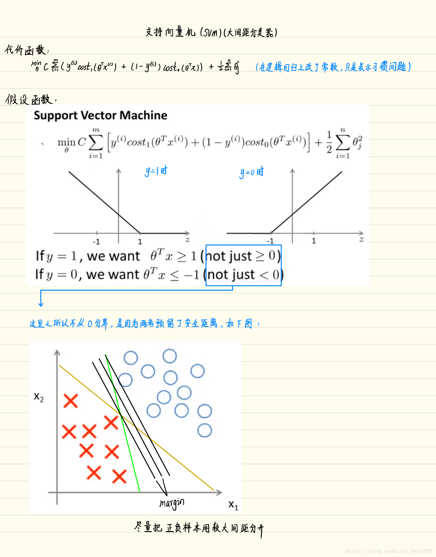

无核SVM
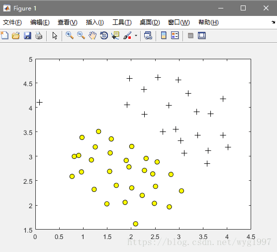
数据可视化:
Code(命令行):
% Load from ex6data1:
% You will have X, y in your environment
load('ex6data1.mat');

% Plot training data
plotData(X, y);
效果图:
训练
Code(这个是写好的代码,码一下以后可以直接用):
function [model] = svmTrain(X, Y, C, kernelFunction, ...
                            tol, max_passes)
%SVMTRAIN Trains an SVM classifier using a simplified version of the SMO
%algorithm.
%   [model] = SVMTRAIN(X, Y, C, kernelFunction, tol, max_passes) trains an
%   SVM classifier and returns trained model. X is the matrix of training
%   examples.  Each row is a training example, and the jth column holds the
%   jth feature.  Y is a column matrix containing 1 for positive examples
%   and 0 for negative examples.  C is the standard SVM regularization
%   parameter.  tol is a tolerance value used for determining equality of
%   floating point numbers. max_passes controls the number of iterations
%   over the dataset (without changes to alpha) before the algorithm quits.
%
% Note: This is a simplified version of the SMO algorithm for training
%       SVMs. In practice, if you want to train an SVM classifier, we
%       recommend using an optimized package such as:
%
%           LIBSVM   (http://www.csie.ntu.edu.tw/~cjlin/libsvm/)
%           SVMLight (http://svmlight.joachims.org/)
%
%

if ~exist('tol', 'var') || isempty(tol)
    tol = 1e-3;
end

if ~exist('max_passes', 'var') || isempty(max_passes)
    max_passes = 5;
end

% Data parameters
m = size(X, 1);
n = size(X, 2);

% Map 0 to -1
Y(Y==0) = -1;

% Variables
alphas = zeros(m, 1);
b = 0;
E = zeros(m, 1);
passes = 0;
eta = 0;
L = 0;
H = 0;

% Pre-compute the Kernel Matrix since our dataset is small
% (in practice, optimized SVM packages that handle large datasets
%  gracefully will _not_ do this)
%
% We have implemented optimized vectorized version of the Kernels here so
% that the svm training will run faster.
if strcmp(func2str(kernelFunction), 'linearKernel')
    % Vectorized computation for the Linear Kernel
    % This is equivalent to computing the kernel on every pair of examples
    K = X*X';
elseif strfind(func2str(kernelFunction), 'gaussianKernel')
    % Vectorized RBF Kernel
    % This is equivalent to computing the kernel on every pair of examples
    X2 = sum(X.^2, 2);
    K = bsxfun(@plus, X2, bsxfun(@plus, X2', - 2 * (X * X')));
    K = kernelFunction(1, 0) .^ K;
else
    % Pre-compute the Kernel Matrix
    % The following can be slow due to the lack of vectorization
    K = zeros(m);
    for i = 1:m
        for j = i:m
             K(i,j) = kernelFunction(X(i,:)', X(j,:)');
             K(j,i) = K(i,j); %the matrix is symmetric
        end
    end
end

% Train
fprintf('\nTraining ...');
dots = 12;
while passes < max_passes,

    num_changed_alphas = 0;
    for i = 1:m,

        % Calculate Ei = f(x(i)) - y(i) using (2).
        % E(i) = b + sum (X(i, :) * (repmat(alphas.*Y,1,n).*X)') - Y(i);
        E(i) = b + sum (alphas.*Y.*K(:,i)) - Y(i);

        if ((Y(i)*E(i) < -tol && alphas(i) < C) || (Y(i)*E(i) > tol && alphas(i) > 0)),

            % In practice, there are many heuristics one can use to select
            % the i and j. In this simplified code, we select them randomly.
            j = ceil(m * rand());
            while j == i,  % Make sure i \neq j
                j = ceil(m * rand());
            end

            % Calculate Ej = f(x(j)) - y(j) using (2).
            E(j) = b + sum (alphas.*Y.*K(:,j)) - Y(j);

            % Save old alphas
            alpha_i_old = alphas(i);
            alpha_j_old = alphas(j);

            % Compute L and H by (10) or (11).
            if (Y(i) == Y(j)),
                L = max(0, alphas(j) + alphas(i) - C);
                H = min(C, alphas(j) + alphas(i));
            else
                L = max(0, alphas(j) - alphas(i));
                H = min(C, C + alphas(j) - alphas(i));
            end

            if (L == H),
                % continue to next i.
                continue;
            end

            % Compute eta by (14).
            eta = 2 * K(i,j) - K(i,i) - K(j,j);
            if (eta >= 0),
                % continue to next i.
                continue;
            end

            % Compute and clip new value for alpha j using (12) and (15).
            alphas(j) = alphas(j) - (Y(j) * (E(i) - E(j))) / eta;

            % Clip
            alphas(j) = min (H, alphas(j));
            alphas(j) = max (L, alphas(j));

            % Check if change in alpha is significant
            if (abs(alphas(j) - alpha_j_old) < tol),
                % continue to next i.
                % replace anyway
                alphas(j) = alpha_j_old;
                continue;
            end

            % Determine value for alpha i using (16).
            alphas(i) = alphas(i) + Y(i)*Y(j)*(alpha_j_old - alphas(j));

            % Compute b1 and b2 using (17) and (18) respectively.
            b1 = b - E(i) ...
                 - Y(i) * (alphas(i) - alpha_i_old) *  K(i,j)' ...
                 - Y(j) * (alphas(j) - alpha_j_old) *  K(i,j)';
            b2 = b - E(j) ...
                 - Y(i) * (alphas(i) - alpha_i_old) *  K(i,j)' ...
                 - Y(j) * (alphas(j) - alpha_j_old) *  K(j,j)';

            % Compute b by (19).
            if (0 < alphas(i) && alphas(i) < C),
                b = b1;
            elseif (0 < alphas(j) && alphas(j) < C),
                b = b2;
            else
                b = (b1+b2)/2;
            end

            num_changed_alphas = num_changed_alphas + 1;

        end

    end

    if (num_changed_alphas == 0),
        passes = passes + 1;
    else
        passes = 0;
    end

    fprintf('.');
    dots = dots + 1;
    if dots > 78
        dots = 0;
        fprintf('\n');
    end
    if exist('OCTAVE_VERSION')
        fflush(stdout);
    end
end
fprintf(' Done! \n\n');

% Save the model
idx = alphas > 0;
model.X= X(idx,:);
model.y= Y(idx);
model.kernelFunction = kernelFunction;
model.b= b;
model.alphas= alphas(idx);
model.w = ((alphas.*Y)'*X)';

end
命令行运行一下,看分类的效果:
C = 1;
model = svmTrain(X, y, C, @linearKernel, 1e-3, 20);
visualizeBoundaryLinear(X, y, model);
我们改变一下C的值,看看效果:
C=1: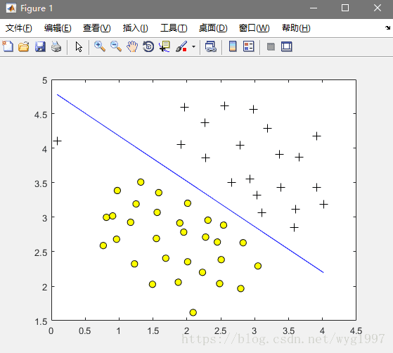
C=100: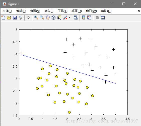
C=0.1: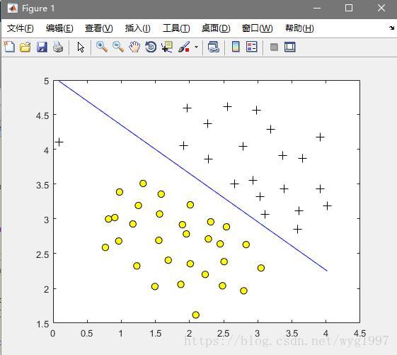
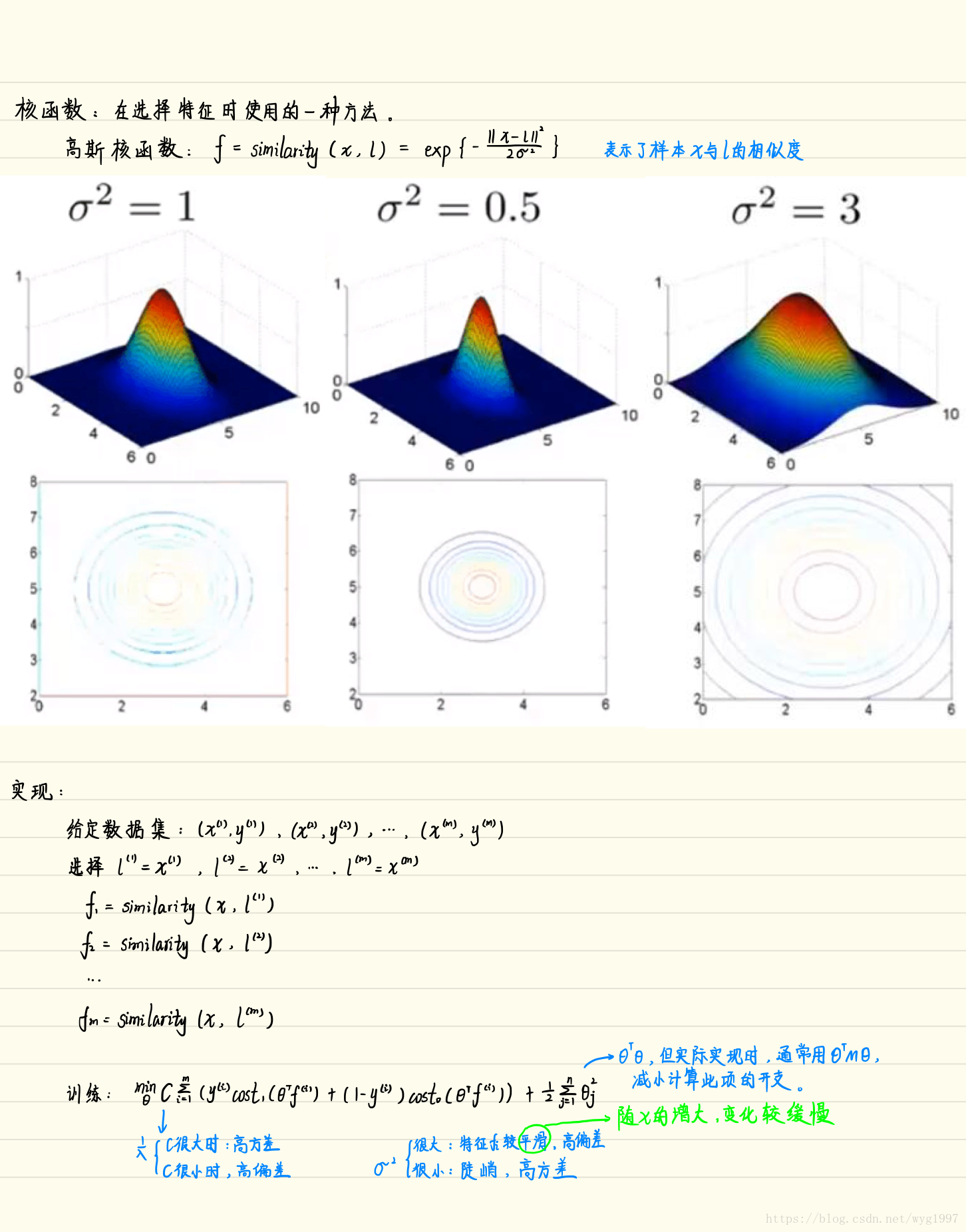
带高斯内核的SVM
内核公式:
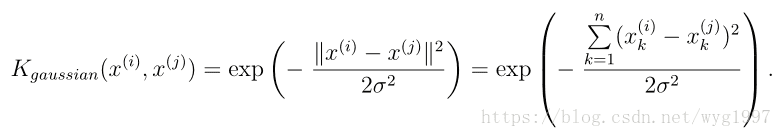
实现一下高斯核的计算:
function sim = gaussianKernel(x1, x2, sigma)
%RBFKERNEL returns a radial basis function kernel between x1 and x2
% sim = gaussianKernel(x1, x2) returns a gaussian kernel between x1 and x2
% and returns the value in sim
% Ensure that x1 and x2 are column vectors
x1 = x1(:); x2 = x2(:);
% You need to return the following variables correctly.
sim = 0;
% ====================== YOUR CODE HERE ======================
% Instructions: Fill in this function to return the similarity between x1
% and x2 computed using a Gaussian kernel with bandwidth
% sigma
%
%
x = x1-x2;
sim = exp(-(x'*x)/(2*sigma*sigma));
% =============================================================
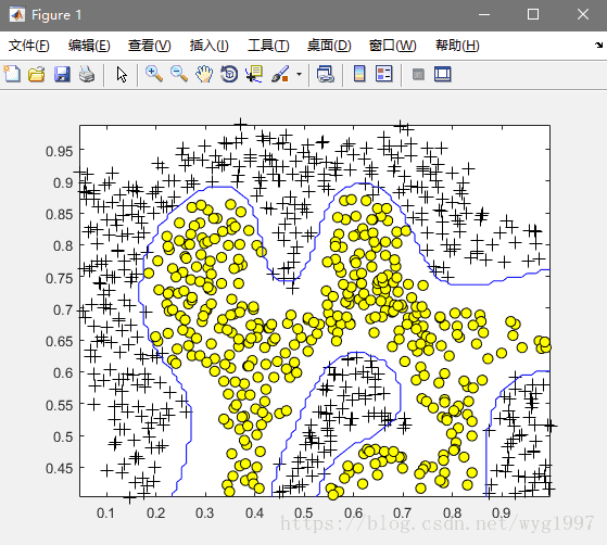
end看一下带高斯核的SVM的分类效果:
Code(命令行运行以下代码):
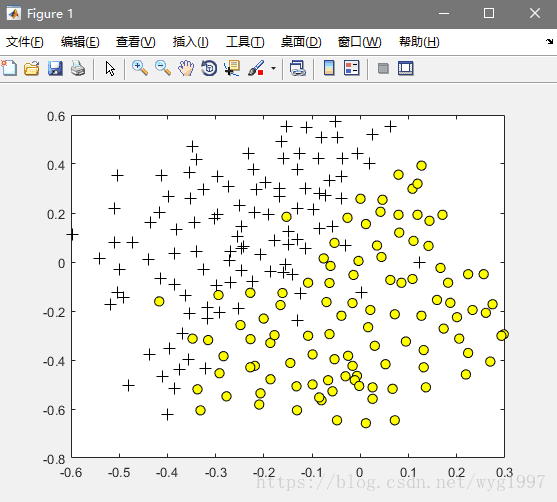
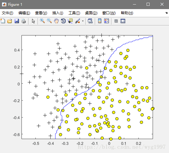
load('ex6data2.mat');

% SVM Parameters
C = 1; sigma = 0.1;

% We set the tolerance and max_passes lower here so that the code will run
% faster. However, in practice, you will want to run the training to
% convergence.
model= svmTrain(X, y, C, @(x1, x2) gaussianKernel(x1, x2, sigma));
visualizeBoundary(X, y, model);
效果图:
关于参数C和λ的选取:
我们用一个新的训练集来介绍这个问题,运行:
% Load from ex6data3:
% You will have X, y in your environment
load('ex6data3.mat');

% Plot training data
plotData(X, y);
效果图:
这里我们用函数来自动选择一个合适的C和λ值(dataset3Params.m):
function [C, sigma] = dataset3Params(X, y, Xval, yval)
%DATASET3PARAMS returns your choice of C and sigma for Part 3 of the exercise
%where you select the optimal (C, sigma) learning parameters to use for SVM
%with RBF kernel
%   [C, sigma] = DATASET3PARAMS(X, y, Xval, yval) returns your choice of C and
%   sigma. You should complete this function to return the optimal C and
%   sigma based on a cross-validation set.
%

% You need to return the following variables correctly.
C = 1;
sigma = 0.3;

% ====================== YOUR CODE HERE ======================
% Instructions: Fill in this function to return the optimal C and sigma
%               learning parameters found using the cross validation set.
%               You can use svmPredict to predict the labels on the cross
%               validation set. For example,
%                   predictions = svmPredict(model, Xval);
%               will return the predictions on the cross validation set.
%
%  Note: You can compute the prediction error using
%        mean(double(predictions ~= yval))
%

%初始化错误率为100%
wrong = 1;

%依次枚举并更新
eg = [0.01, 0.03, 0.1, 0.3, 1, 3, 10, 30];
for i = 1:length(eg)
    for j = 1:length(eg)
        model= svmTrain(X, y, eg(i), @(x1, x2) gaussianKernel(x1, x2, eg(j)));
        predictions = svmPredict(model, Xval);
        twrong = mean(double(predictions ~= yval));

        %如果得到的错误率更小,就更新
        if (twrong < wrong)
            wrong = twrong;
            C = eg(i);
            sigma = eg(j);
        end
    end
end

% =========================================================================

end
然后再画图看看,运行:
model= svmTrain(X, y, C, @(x1, x2) gaussianKernel(x1, x2, sigma));
visualizeBoundary(X, y, model);
效果:
最后码一下预测的函数(svmPredict.m):
function pred = svmPredict(model, X)
%SVMPREDICT returns a vector of predictions using a trained SVM model
%(svmTrain).
%   pred = SVMPREDICT(model, X) returns a vector of predictions using a
%   trained SVM model (svmTrain). X is a mxn matrix where there each
%   example is a row. model is a svm model returned from svmTrain.
%   predictions pred is a m x 1 column of predictions of {0, 1} values.
%

% Check if we are getting a column vector, if so, then assume that we only
% need to do prediction for a single example
if (size(X, 2) == 1)
    % Examples should be in rows
    X = X';
end

% Dataset
m = size(X, 1);
p = zeros(m, 1);
pred = zeros(m, 1);

if strcmp(func2str(model.kernelFunction), 'linearKernel')
    % We can use the weights and bias directly if working with the
    % linear kernel
    p = X * model.w + model.b;
elseif strfind(func2str(model.kernelFunction), 'gaussianKernel')
    % Vectorized RBF Kernel
    % This is equivalent to computing the kernel on every pair of examples
    X1 = sum(X.^2, 2);
    X2 = sum(model.X.^2, 2)';
    K = bsxfun(@plus, X1, bsxfun(@plus, X2, - 2 * X * model.X'));
    K = model.kernelFunction(1, 0) .^ K;
    K = bsxfun(@times, model.y', K);
    K = bsxfun(@times, model.alphas', K);
    p = sum(K, 2);
else
    % Other Non-linear kernel
    for i = 1:m
        prediction = 0;
        for j = 1:size(model.X, 1)
            prediction = prediction + ...
                model.alphas(j) * model.y(j) * ...
                model.kernelFunction(X(i,:)', model.X(j,:)');
        end
        p(i) = prediction + model.b;
    end
end

% Convert predictions into 0 / 1
pred(p >= 0) =  1;
pred(p <  0) =  0;

end