文章目录
欢迎关注我的 微信公众号:破壳Ai,分享最佳学习路径、教程和资源。成长路上,有我陪你。
支持向量机
在本练习中,我们将使用高斯核函数的支持向量机(SVM)来构建垃圾邮件分类器。
数据集
import numpy as np
import pandas as pd
import matplotlib.pyplot as plt
from scipy.io import loadmat
path = '数据集/ex6data1.mat'
raw_data = loadmat(path)
data = pd.DataFrame(raw_data['X'], columns=['X1', 'X2'])
data['y'] = raw_data['y']
data.head()
| X1 | X2 | y | |
|---|---|---|---|
| 0 | 1.9643 | 4.5957 | 1 |
| 1 | 2.2753 | 3.8589 | 1 |
| 2 | 2.9781 | 4.5651 | 1 |
| 3 | 2.9320 | 3.5519 | 1 |
| 4 | 3.5772 | 2.8560 | 1 |
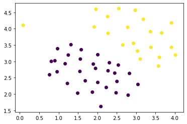
# 绘制图像
plt.scatter(data.X1, data.X2, c=data.y)
plt.show()
# 用plot库绘制
def plot_init_pic(data, fig, ax):
    positive = data.loc[data['y']==1]
    negative = data.loc[data['y']==0]

    ax.scatter(positive['X1'], positive['X2'], s=50, marker='+', label='Positive')
    ax.scatter(negative['X1'], negative['X2'], s=50, marker='o', label='Negative')
fig, ax = plt.subplots(figsize=(12, 8))
plot_init_pic(data, fig, ax)
ax.set_xlabel('X1')
ax.set_ylabel('X2')
ax.legend()
plt.show()
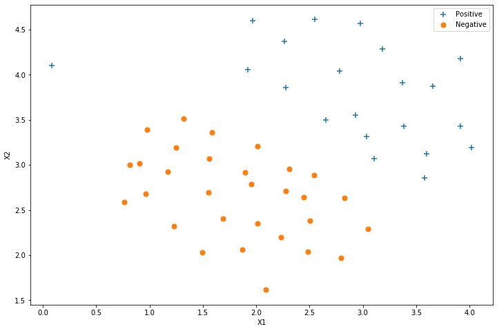
请注意,还有一个异常的正例在其他样本之外。
这些类仍然是线性分离的,但它非常紧凑。 我们要训练线性支持向量机来学习类边界。
try C = 1
from sklearn import svm

# 配置LinearSVC参数
svc = svm.LinearSVC(C=1, loss='hinge', max_iter=20000)
svc
LinearSVC(C=1, class_weight=None, dual=True, fit_intercept=True,
          intercept_scaling=1, loss='hinge', max_iter=20000, multi_class='ovr',
          penalty='l2', random_state=None, tol=0.0001, verbose=0)
# 将之前配置好的模型应用到数据集上
svc.fit(data[['X1', 'X2']], data['y'])
svc.score(data[['X1', 'X2']], data['y'])
0.9803921568627451
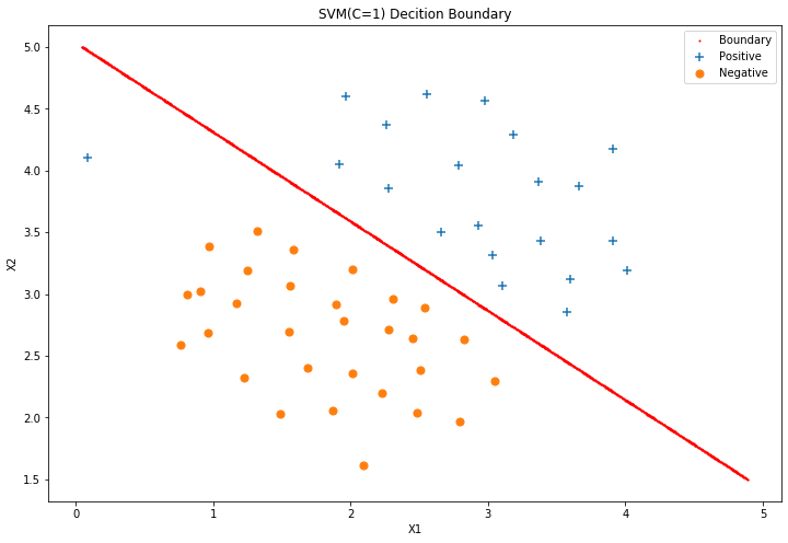
找出决策边界再绘制
# 法一: 组建网格然后将网格点带入决策边界函数,找出值近似为0的点就是边界点
def find_decision_boundary(svc, x1min, x1max, x2min, x2max, diff):
    x1 = np.linspace(x1min, x1max, 1000)
    x2 = np.linspace(x2min, x2max, 1000)

    coordinates = [(x, y) for x in x1 for y in x2]
    x_cord, y_cord = zip(*coordinates)
    c_val = pd.DataFrame({

    'x1':x_cord, 'x2':y_cord})
    c_val['val'] = svc.decision_function(c_val[['x1', 'x2']])

    decision = c_val[np.abs(c_val['val']) < diff]

    return decision.x1, decision.x2
x1, x2 = find_decision_boundary(svc, 0, 5, 1.5, 5, 2 * 10**-3)

# fig. ax = plt.subplots(figsize=(12, 8))  逗号写成了点,jupyter发现不了
fig, ax = plt.subplots(figsize=(12, 8))
ax.scatter(x1, x2, s=1, c='r', label='Boundary')

plot_init_pic(data, fig, ax)

ax.set_title('SVM(C=1) Decition Boundary')
ax.set_xlabel('X1')
ax.set_ylabel('X2')
ax.legend()

plt.show()
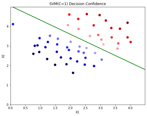
# The confidence score for a sample is the signed distance of that sample to the hyperplane.
data['SVM1 Confidence'] = svc.decision_function(data[['X1', 'X2']])
fig, ax = plt.subplots(figsize=(8, 6))
ax.scatter(data['X1'], data['X2'], s=50, c=data['SVM1 Confidence'], cmap='seismic')
ax.set_title('SVM(C=1) Decision Confidence')
ax.set_xlabel('X1')
ax.set_ylabel('X2')

# 法二:决策边界, 使用等高线表示
x1 = np.arange(0, 4.5, 0.01)
x2 = np.arange(0, 5, 0.01)
x1, x2 = np.meshgrid(x1, x2)
y_pred = np.array([svc.predict(np.vstack((a, b)).T) for (a, b) in zip(x1, x2)])
plt.contour(x1, x2, y_pred, colors='g', linewidths=1)

plt.show()

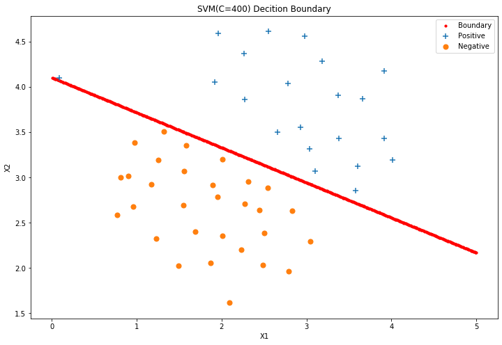
try C = 400
C对应正则化的 λ \lambda λ, C = 1 λ C = \frac{1}{\lambda} C=λ1,C越大越容易过拟合。图像中最左侧的点被划分到右侧。
svc1 = svm.LinearSVC(C=400, loss='hinge', max_iter=20000)
svc1.fit(data[['X1', 'X2']], data['y'])
svc1.score(data[['X1', 'X2']], data['y'])
C:\Users\humin\anaconda3\lib\site-packages\sklearn\svm\_base.py:947: ConvergenceWarning: Liblinear failed to converge, increase the number of iterations.
  "the number of iterations.", ConvergenceWarning)


1.0
决策边界
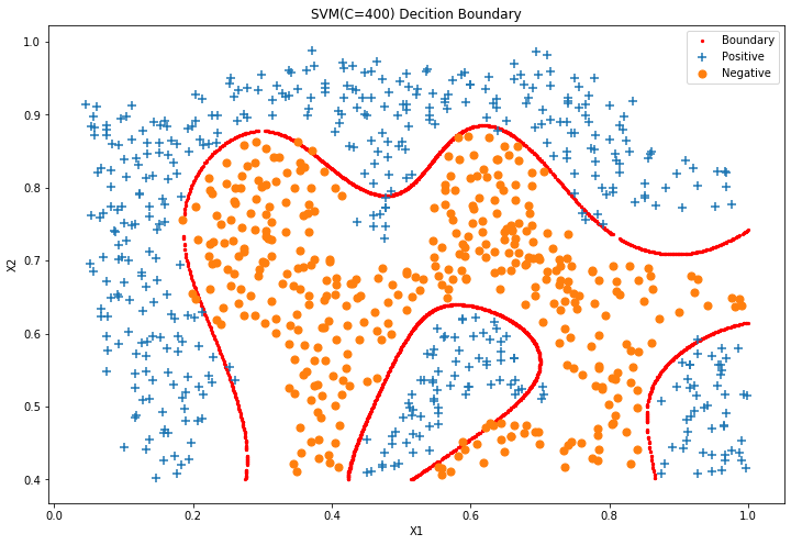
x1, x2 = find_decision_boundary(svc1, 0, 5, 1.5, 5, 8 * 10**-3)  # 这里调整了diff这个阈值,否则决策点连不成一条连续的线

fig, ax = plt.subplots(figsize=(12, 8))
ax.scatter(x1, x2, s=10, c='r', label='Boundary')

plot_init_pic(data, fig, ax)

ax.set_title('SVM(C=400) Decition Boundary')
ax.set_xlabel('X1')
ax.set_ylabel('X2')
ax.legend()

plt.show()
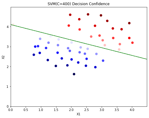
# The confidence score for a sample is the signed distance of that sample to the hyperplane.
data['SVM400 Confidence'] = svc1.decision_function(data[['X1', 'X2']])
fig, ax = plt.subplots(figsize=(8, 6))
ax.scatter(data['X1'], data['X2'], s=50, c=data['SVM400 Confidence'], cmap='seismic')
ax.set_title('SVM(C=400) Decision Confidence')
ax.set_xlabel('X1')
ax.set_ylabel('X2')

# 决策边界, 使用等高线表示
x1 = np.arange(0, 4.5, 0.01)
x2 = np.arange(0, 5, 0.01)
x1, x2 = np.meshgrid(x1, x2)
y_pred = np.array([svc1.predict(np.vstack((a, b)).T) for (a, b) in zip(x1, x2)])
plt.contour(x1, x2, y_pred, colors='g', linewidths=.5)

plt.show()
高斯核函数 SVM with Gaussian Kernels
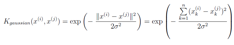
def gaussian_kernel(x1, x2, sigma):
    return np.exp(-np.power(x1-x2, 2).sum() / (2 * sigma**2))
x1 = np.array([1, 2, 1])
x2 = np.array([0, 4, -1])
sigma = 2

gaussian_kernel(x1, x2, sigma)
0.32465246735834974
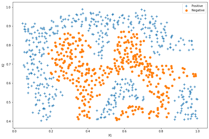
数据集2
接下来,在另一个数据集上使用高斯内核,找非线性边界。
raw_data = loadmat('数据集/ex6data2.mat')
data = pd.DataFrame(raw_data['X'], columns=['X1', 'X2'])
data['y'] = raw_data['y']
fig, ax = plt.subplots(figsize=(12, 8))
plot_init_pic(data, fig, ax)
ax.set_xlabel('X1')
ax.set_ylabel('X2')
ax.legend()
plt.show()
svc2 = svm.SVC(C=100, gamma=10, probability=True)
svc2
SVC(C=100, break_ties=False, cache_size=200, class_weight=None, coef0=0.0,
    decision_function_shape='ovr', degree=3, gamma=10, kernel='rbf',
    max_iter=-1, probability=True, random_state=None, shrinking=True, tol=0.001,
    verbose=False)
svc2.fit(data[['X1', 'X2']], data['y'])
svc2.score(data[['X1', 'X2']], data['y'])
0.9698725376593279
直接绘制决策边界
# 法二:利用等高线绘制决策边界
def plot_decision_boundary(svc, x1min, x1max, x2min, x2max, ax):
#     x1 = np.arange(x1min, x1max, 0.001)
#     x2 = np.arange(x2min, x2max, 0.001)
    x1 = np.linspace(x1min, x1max, 1000)
    x2 = np.linspace(x2min, x2max, 1000)

    x1, x2 = np.meshgrid(x1, x2)
    y_pred = np.array([svc.predict(np.vstack((a, b)).T) for (a, b) in zip(x1, x2)])

    ax.contour(x1, x2, y_pred, colors='r', linewidths=5)
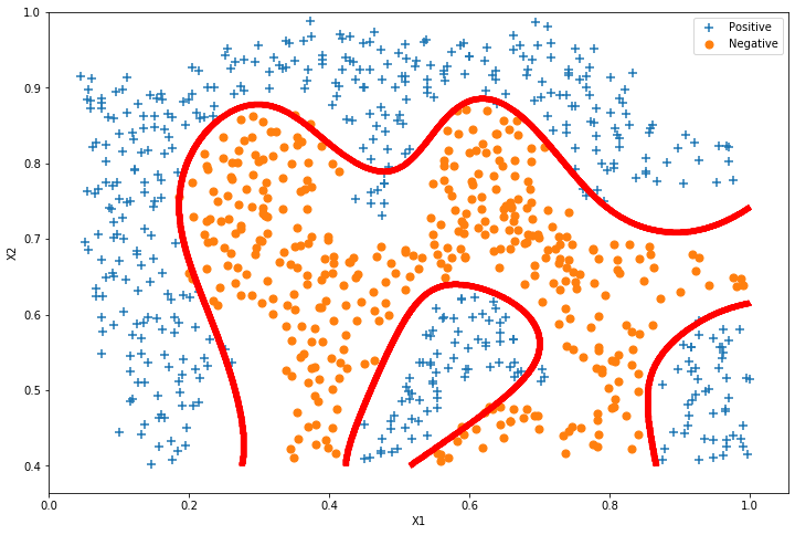
fig, ax = plt.subplots(figsize=(12, 8))

plot_init_pic(data, fig, ax)
plot_decision_boundary(svc2, 0, 1, 0.4, 1, ax)

ax.set_xlabel('X1')
ax.set_ylabel('X2')
ax.legend()
plt.show()

# 10秒
# 法一 要15秒
x1, x2 = find_decision_boundary(svc2, 0, 1, 0.4, 1, 0.01)  # 这里调整了diff这个阈值,否则决策点连不成一条连续的线

fig, ax = plt.subplots(figsize=(12, 8))
ax.scatter(x1, x2, s=5, c='r', label='Boundary')

plot_init_pic(data, fig, ax)

ax.set_title('SVM(C=400) Decition Boundary')
ax.set_xlabel('X1')
ax.set_ylabel('X2')
ax.legend()

plt.show()
数据集3
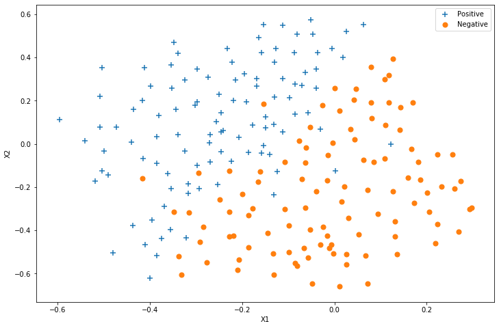
对于第三个数据集,我们给出了训练和验证集,并且基于验证集性能为SVM模型找到最优超参数。
我们现在需要寻找最优和,候选数值为[0.01, 0.03, 0.1, 0.3, 1, 3, 10, 30, 100]
raw_data = loadmat('数据集/ex6data3.mat')
data = pd.DataFrame(raw_data['X'], columns=['X1', 'X2'])
data['y'] = raw_data['y']

Xval = raw_data['Xval']
yval = raw_data['yval']
fig, ax = plt.subplots(figsize=(12, 8))
plot_init_pic(data, fig, ax)
ax.set_xlabel('X1')
ax.set_ylabel('X2')
ax.legend()
plt.show()
找最优超参数
C_values = [0.01, 0.03, 0.1, 0.3, 1, 3, 10, 30, 100]
gamma_values = [0.01, 0.03, 0.1, 0.3, 1, 3, 10, 30, 100]

best_score = 0
best_params = {

    'C':None, 'gamma':None}
for c in C_values:
    for gamma in gamma_values:
        svc = svm.SVC(C=c, gamma=gamma, probability=True)
        svc.fit(data[['X1', 'X2']], data['y']) # 用训练集训练
        score =  svc.score(Xval, yval)  # 用验证集选优
        if score > best_score:
            best_score = score
            best_params['C'] = c
            best_params['gamma'] = gamma
best_score, best_params
(0.965, {'C': 0.3, 'gamma': 100})
绘制决策曲线
svc3 = svm.SVC(C=best_params['C'], gamma=best_params['gamma'], probability=True)
svc3
SVC(C=0.3, break_ties=False, cache_size=200, class_weight=None, coef0=0.0,
    decision_function_shape='ovr', degree=3, gamma=100, kernel='rbf',
    max_iter=-1, probability=True, random_state=None, shrinking=True, tol=0.001,
    verbose=False)
svc3.fit(data[['X1', 'X2']], data['y'])
svc3.score(data[['X1', 'X2']], data['y'])
0.95260663507109
fig, ax = plt.subplots(figsize=(12, 8))

plot_init_pic(data, fig, ax)
plot_decision_boundary(svc3, -0.6, 0.3, -0.7, 0.6, ax)

ax.set_xlabel('X1')
ax.set_ylabel('X2')
ax.legend()
plt.show()

垃圾邮件处理
在这一部分中,我们的目标是使用SVM来构建垃圾邮件过滤器。
特征提取的思路:
首先对垃圾邮件进行预处理:
Lower-casing
Stripping HTML
Normalizing URLs
Normalizing Email Addresses
Normalizing Numbers
Normalizing Dollars
Word Stemming
Removal of non-words
然后统计所有的垃圾邮件中单词出现的频率,提取频率超过100次的单词,得到一个单词列表。
将每个单词替换为列表中对应的编号。
提取特征:每个邮件对应一个n维向量 R n R^n Rn, x i ∈ 0 , 1 x_i \in {0, 1} xi∈0,1,如果第i个单词出现,则 x i = 1 x_i=1 xi=1,否则 x i = 0 x_i=0 xi=0
本文偷懒直接使用已经处理好的特征和数据…
spam_train = loadmat('数据集/spamTrain.mat')
spam_test = loadmat('数据集/spamTest.mat')

spam_train
spam_train.keys(), spam_test.keys()   # 这个好,不用把所有数据打印出来就能直接看到数据的标签
(dict_keys(['__header__', '__version__', '__globals__', 'X', 'y']),
 dict_keys(['__header__', '__version__', '__globals__', 'Xtest', 'ytest']))
X = spam_train['X']
Xtest = spam_test['Xtest']

y = spam_train['y'].ravel()
ytest = spam_test['ytest'].ravel()

X.shape, y.shape, Xtest.shape, ytest.shape
((4000, 1899), (4000,), (1000, 1899), (1000,))
每个文档已经转换为一个向量,其中1,899个维对应于词汇表中的1,899个单词。 它们的值为二进制,表示文档中是否存在该单词。
svc4 = svm.SVC()
svc4.fit(X, y)
SVC(C=1.0, break_ties=False, cache_size=200, class_weight=None, coef0=0.0,
    decision_function_shape='ovr', degree=3, gamma='scale', kernel='rbf',
    max_iter=-1, probability=False, random_state=None, shrinking=True,
    tol=0.001, verbose=False)
print('Training accuracy = {0}%'.format(np.round(svc4.score(X, y) * 100, 2)))
print('Test accuracy = {0}%'.format(np.round(svc4.score(Xtest, ytest) * 100, 2)))
Training accuracy = 99.32%
Test accuracy = 98.7%
找出垃圾邮件敏感单词
kw = np.eye(1899)  # 为每个单词生成一个向量,每一行代表一个单词
spam_val = pd.DataFrame({

    'idx':range(1899)})

print(kw[:3,:])
[[1. 0. 0. ... 0. 0. 0.]
 [0. 1. 0. ... 0. 0. 0.]
 [0. 0. 1. ... 0. 0. 0.]]
spam_val['isspam'] = svc4.decision_function(kw)

spam_val.head()
| idx | isspam | |
|---|---|---|
| 0 | 0 | -0.093653 |
| 1 | 1 | -0.083078 |
| 2 | 2 | -0.109401 |
| 3 | 3 | -0.119685 |
| 4 | 4 | -0.165824 |
spam_val['isspam'].describe()
count    1899.000000
mean       -0.110039
std         0.049094
min        -0.428396
25%        -0.131213
50%        -0.111985
75%        -0.091973
max         0.396286
Name: isspam, dtype: float64
decision = spam_val[spam_val['isspam'] > 0] # 提取出垃圾邮件敏感单词
decision
| idx | isspam | |
|---|---|---|
| 155 | 155 | 0.095529 |
| 173 | 173 | 0.066666 |
| 297 | 297 | 0.396286 |
| 351 | 351 | 0.023785 |
| 382 | 382 | 0.030317 |
| 476 | 476 | 0.042474 |
| 478 | 478 | 0.057344 |
| 529 | 529 | 0.060692 |
| 537 | 537 | 0.008558 |
| 680 | 680 | 0.109643 |
| 697 | 697 | 0.003269 |
| 738 | 738 | 0.092561 |
| 774 | 774 | 0.181496 |
| 791 | 791 | 0.040396 |
| 1008 | 1008 | 0.012187 |
| 1088 | 1088 | 0.132633 |
| 1101 | 1101 | 0.002832 |
| 1120 | 1120 | 0.003076 |
| 1163 | 1163 | 0.072045 |
| 1178 | 1178 | 0.012122 |
| 1182 | 1182 | 0.015656 |
| 1190 | 1190 | 0.232788 |
| 1263 | 1263 | 0.160806 |
| 1298 | 1298 | 0.044018 |
| 1372 | 1372 | 0.019640 |
| 1397 | 1397 | 0.218337 |
| 1399 | 1399 | 0.018762 |
| 1460 | 1460 | 0.001859 |
| 1467 | 1467 | 0.002822 |
| 1519 | 1519 | 0.001654 |
| 1661 | 1661 | 0.003775 |
| 1721 | 1721 | 0.057241 |
| 1740 | 1740 | 0.034107 |
| 1795 | 1795 | 0.125143 |
| 1823 | 1823 | 0.002071 |
| 1829 | 1829 | 0.002630 |
| 1851 | 1851 | 0.030662 |
| 1892 | 1892 | 0.052786 |
| 1894 | 1894 | 0.101613 |
path = '数据集/vocab.txt'
voc = pd.read_csv(path, header=None, names=['idx', 'voc'], sep='\t')
voc.head()
| idx | voc | |
|---|---|---|
| 0 | 1 | aa |
| 1 | 2 | ab |
| 2 | 3 | abil |
| 3 | 4 | abl |
| 4 | 5 | about |
spamvoc = voc.loc[decision['idx']]

spamvoc
| idx | voc | |
|---|---|---|
| 155 | 156 | basenumb |
| 173 | 174 | below |
| 297 | 298 | click |
| 351 | 352 | contact |
| 382 | 383 | credit |
| 476 | 477 | dollar |
| 478 | 479 | dollarnumb |
| 529 | 530 | |
| 537 | 538 | encod |
| 680 | 681 | free |
| 697 | 698 | futur |
| 738 | 739 | guarante |
| 774 | 775 | here |
| 791 | 792 | hour |
| 1008 | 1009 | market |
| 1088 | 1089 | nbsp |
| 1101 | 1102 | nextpart |
| 1120 | 1121 | numbera |
| 1163 | 1164 | offer |
| 1178 | 1179 | opt |
| 1182 | 1183 | order |
| 1190 | 1191 | our |
| 1263 | 1264 | pleas |
| 1298 | 1299 | price |
| 1372 | 1373 | receiv |
| 1397 | 1398 | remov |
| 1399 | 1400 | repli |
| 1460 | 1461 | se |
| 1467 | 1468 | see |
| 1519 | 1520 | sincer |
| 1661 | 1662 | text |
| 1721 | 1722 | transfer |
| 1740 | 1741 | type |
| 1795 | 1796 | visit |
| 1823 | 1824 | websit |
| 1829 | 1830 | welcom |
| 1851 | 1852 | will |
| 1892 | 1893 | you |
| 1894 | 1895 | your |
欢迎关注我的 微信公众号:破壳Ai,分享最佳学习路径、教程和资源。成长路上,有我陪你。