Sequence Model (三)

详细的笔记：
第二周 自然语言处理与词嵌入（Natural Language Processing and Word Embeddings）

Word Representations

One-hot representation 把词与词割裂起来，使得算法对相关词的泛化能力不强。

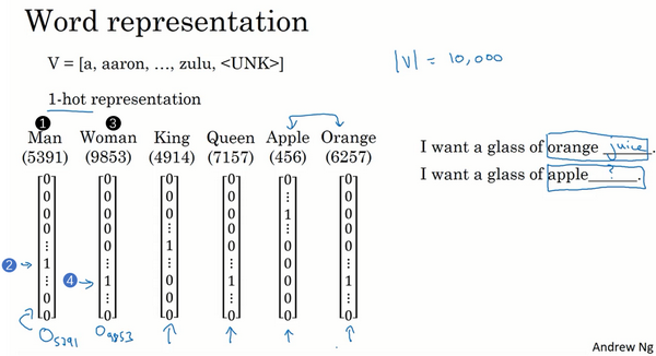
我们希望能够学习到一种表达，使得可以通过词向量在向量空间内的距离来衡量词与词语义上的相似性。


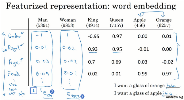
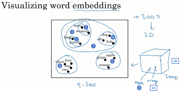
Word embeddings algorithms like this can learn similar features for concepts that feel like they should be more related, as visualized by that concept that seem to you and me like they should be more similar, end up getting mapped to a more similar feature vectors. And these representations will use these sort of featurized representations in maybe a 300 dimensional space, these are called embeddings. And the reason we call them embeddings is, you can think of a 300 dimensional space. And again, they can’t draw out here in two dimensional space because it’s a 3D one. And what you do is you take every words like orange, and have a three dimensional feature vector so that word orange gets embedded to a point in this 300 dimensional space. And the word apple, gets embedded to a different point in this 300 dimensional space.

Using word embeddings

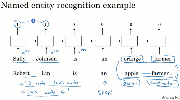
One of the reasons that word embeddings will be able to do this is the algorithms to learning word embeddings can examine very large text corpuses, maybe found off the Internet.

So you can examine very large data sets, maybe a billion words, maybe even up to 100 billion words would be quite reasonable. So very large training sets of just unlabeled text. And by examining tons of unlabeled text, which you can download more or less for free, you can figure out that orange and durian are similar. And farmer and cultivator are similar, and therefore, learn embeddings, that groups them together. Now having discovered that orange and durian are both fruits by reading massive amounts of Internet text, what you can do is then take this word embedding and apply it to your named entity recognition task, for which you might have a much smaller training set, maybe just 100,000 words in your training set, or even much smaller.

And so this allows you to carry out transfer learning, where you take information you've learned from huge amounts of unlabeled text that you can suck down essentially for free off the Internet to figure out that orange, apple, and durian are fruits. And then transfer that knowledge to a task, such as named entity recognition, for which you may have a relatively small labeled training set.

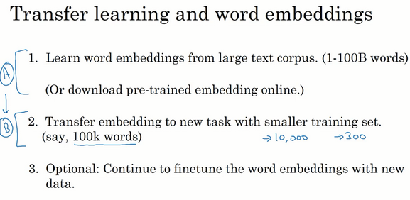
To summarize, this is how you can carry out transfer learning using word embeddings.

• Step 1 is to learn word embeddings from a large text corpus, a very large text corpus or you can also download pre-trained word embeddings online. There are several word embeddings that you can find online under very permissive licenses.

• And you can then take these word embeddings and transfer the embedding to new task, where you have a much smaller labeled training sets. And use this, let’s say, 300 dimensional embedding, to represent your words.

  • One nice thing also about this is you can now use relatively lower dimensional feature vectors. So rather than using a 10,000 dimensional one-hot vector, you can now instead use maybe a 300 dimensional dense vector. Although the one-hot vector is fast and the 300 dimensional vector that you might learn for your embedding will be a dense vector.

• And then, finally, as you train your model on your new task, on your named entity recognition task with a smaller label data set, one thing you can optionally do is to continue to fine tune, continue to adjust the word embeddings with the new data.

  • In practice, you would do this only if this task 2 has a pretty big data set. If your label data set for step 2 is quite small, then usually, I would not bother to continue to fine tune the word embeddings.

So word embeddings tend to make the biggest difference when the task you're trying to carry out has a relatively smaller training set.

What we’ll do for learning word embeddings is that we'll have a fixed vocabulary of, say, 10,000 words. And we'll learn a vector e1 through, say, e10,000 that just learns a fixed encoding or learns a fixed embedding for each of the words in our vocabulary.

Properties of word embeddings

One of the most fascinating properties of word embeddings is that they can also help with analogy reasoning. And while reasonable analogies may not be by itself the most important NLP application, they might also help convey a sense of what these word embeddings are doing, what these word embeddings can do.

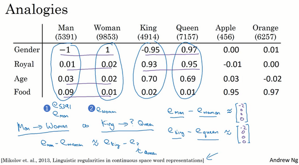
这些向量有一个有趣的特性，就是假如你有向量$e_{\text{man}}$和$e_{\text{woman}}$，将它们进行减法运算，即

$$\begin{align*} e_{\text{man}} - e_{\text{woman}} = \begin{bmatrix} 1 \ 0.01 \ 0.03 \ 0.09 \ \end{bmatrix} - \begin{bmatrix} 1 \ 0.02 \ 0.02 \ 0.01 \ \end{bmatrix} = \begin{bmatrix} 2 \ 0.01 \ 0.01 \ 0.08 \ \end{bmatrix} \approx \begin{bmatrix} 2 \ 0 \ 0 \ 0 \ \end{bmatrix} \end{align*}$$
类似的，假如你用 $e_{\text{king}}$减去 $e_{\text{queen}}$，最后也会得到一样的结果，即
$$\begin{align*} e_{\text{king}} - e_{\text{queen}} = \begin{bmatrix} 0.95 \ 0.93 \ 0.70 \ 0.02 \ \end{bmatrix} - \begin{bmatrix} 0.97 \ 0.95 \ 0.69 \ 0.01 \ \end{bmatrix} = \begin{bmatrix}1.92 \ 0.02 \ 0.01 \ 0.01 \ \end{bmatrix} \approx \begin{bmatrix} 2 \ 0 \ 0 \ 0 \ \end{bmatrix} \end{align*}$$
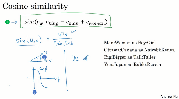
这个结果表示，man和woman主要的差异是gender（性别）上的差异，而king和queen之间的主要差异，根据向量的表示，也是gender（性别）上的差异，这就是为什么 $e_{\text{man}}- e_{\text{woman}}$和 $e_{\text{king}} - e_{\text{queen}}$结果是相同的。所以得出这种类比推理的结论的方法就是，当算法被问及man对woman相当于king对什么时，算法所做的就是计算 $e_{\text{man}}-e_{\text{woman}}$，然后找出一个向量也就是找出一个词，使得 $e_{\text{man}}-e_{\text{woman}}$≈ $\ e_{\text{king}}- e_{?}$，也就是说，当这个新词是queen时，式子的左边会近似地等于右边。

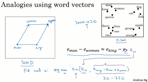
In pictures, the word embeddings live in maybe a 300 dimensional space. And so the word man is represented as a point in the space, and the word woman is represented as a point in the space. And the word king is represented as another point, and the word queen is represented as another point. And what we pointed out really on the last slide is that the vector difference between man and woman is very similar to the vector
difference between king and queen.

Embedding matrix

When you implement an algorithm to learn a word embedding, what you end up learning is an embedding matrix.

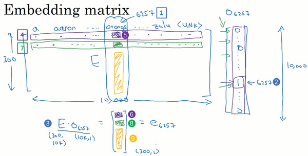
That’s why the embedding matrix $E$ times this one-hot vector here winds up selecting out this 300-dimensional column corresponding to the word Orange.

The thing to remember from this slide is that our goal will be to learn an embedding matrix $E$.

Learning word embeddings

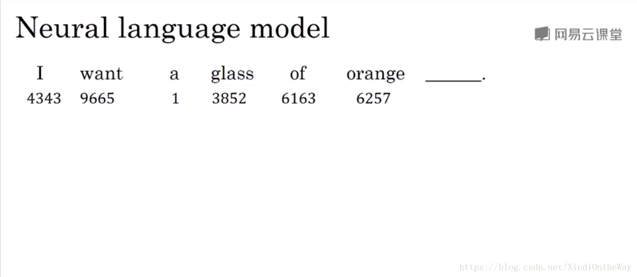
Let’s say you’re building a language model and you do it with a neural network. So, during training, you might want your neural network to do something like input, I want a glass of orange, and then predict the next word in the sequence. And below each of these words, I have also written down the index in the vocabulary of the different words.

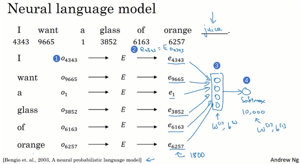
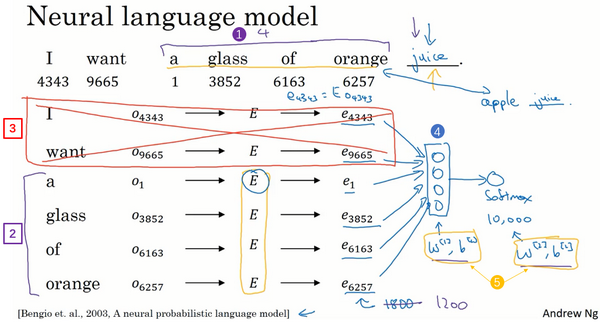
Well, what’s actually more commonly done is to have a fixed historical window. So for example, you might decide that you always want to predict the next word given say the previous four words, where four here is a hyperparameter of the algorithm. So this is how you adjust to either very long or very short sentences or you decide to always just look at the previous four words, so you say, I will still use those four words. And so, let’s just get rid of these. And so, if you’re always using a four word history, this means that your neural network will input a 1,200 dimensional feature vector, go into this layer, then have a softmax and try to predict the output.

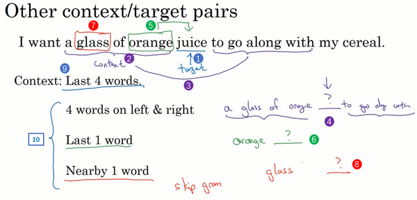
And so, if your goal is to learn a embedding of researchers I’ve experimented with many different types of context. If it goes to build a language model then is natural for the context to be a few words right before the target word. But if your goal is not to learn the language model, then you can choose other contexts. For example, you can pose a learning problem where the context is the four words on the left and right. So, you can take the four words on the left and right as the context, and what that means is that we’re posing a learning problem where the algorithm is given four words on the left. So, a glass of orange, and four words on the right, to go along with, and this has to predict the word in the middle. And posing a learning problem like this where you have the embeddings of the left four words and the right four words feed into a neural network, similar to what you saw in the previous slide, to try to predict the word in the middle, try to put it target word in the middle, this can also be used to learn word embeddings.

word2vec

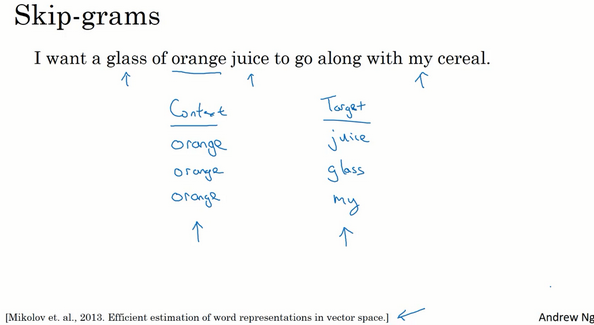
In the skip-gram model, what we’re going to do is come up with a few context to target word to create our supervised learning problem.

So rather than having the context be always the last four words or the last end words immediately before the target word, what I’m going to do is, say, randomly pick a word to be the context word. And let’s say we chose the word orange. And what we’re going to do is randomly pick another word within some window. Say plus minus five words or plus minus ten words of the context word and we choose that to be target word. So maybe just by chance you might pick juice to be a target word, that’s just one word later. Or you might choose two words before. So you have another pair where the target could be glass or, Maybe just by chance you choose
the word my as the target. And so we’ll set up a supervised learning problem where given the context word, you're asked to predict what is a randomly chosen word within say, a plus minus ten word window, or plus minus five or ten word window of that input context word.

But the goal that’s setting up this supervised learning problem, isn’t to do well on the supervised learning problem itself, it is that we want to use this learning problem to learn good word embeddings.

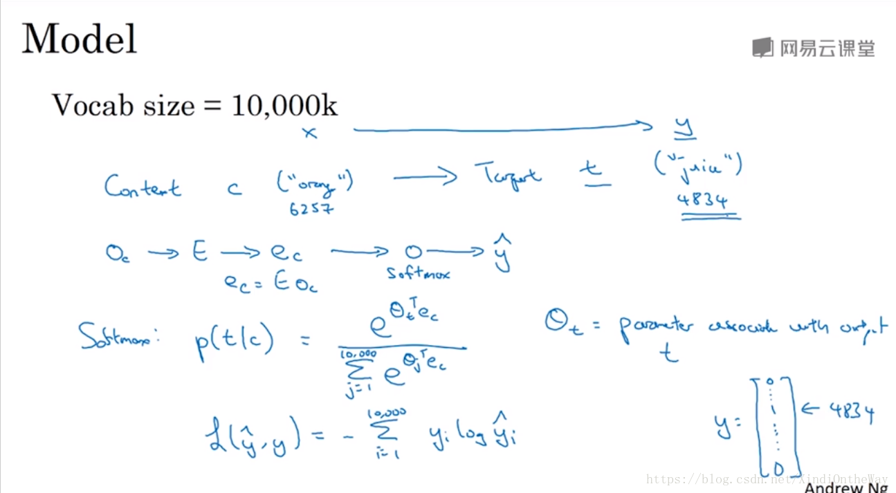
Let’s say that we’ll continue to our vocab of 10,000 words.
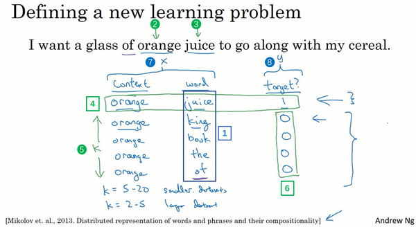
The basic supervised learning problem we’re going to solve is that we want to learn the mapping from some Context c, such as the word "orange" to some target, which we will call t, which might be the word "juice" or the word "glass" or the word "my".

If we use the example from the previous slide. So in our vocabulary, “orange” is word 6257, and the word “juice” is the word 4834 in our vocab of 10,000 words. And so that’s the input x that you want to learn to map to that output y.

$$O_c \rightarrow E \rightarrow e_c=EO_c \rightarrow softmax \rightarrow \hat{y}$$

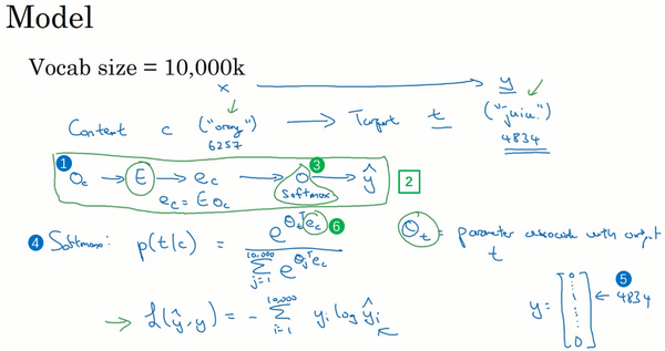
So to summarize, this is the overall little model, little neural network with basically looking up the embedding and then just a softmax unit. And the matrix $E$ will have a lot of parameters, so the matrix $E$ has parameters corresponding to all of these embedding vectors, $e_c$. And then the softmax unit also has parameters that gives the $\theta_t$ parameters but if you optimize this loss function with respect to the all of these parameters, you actually get a pretty good set of embedding vectors.

So this is called the skip-gram model because is taking as input one word like orange and then trying to predict some words skipping a few words from the left or the right side. To predict what comes little bit before little bit after the context words.

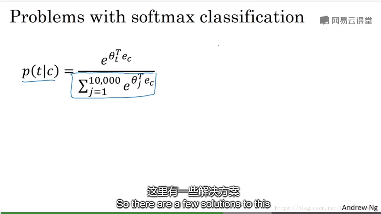
And the primary problem is computational speed. In particular, for the softmax model, every time you want to evaluate this probability, you need to carry out a sum over all 10,000 words in your vocabulary. And maybe 10,000 isn’t too bad, but if you’re using a vocabulary of size 100,000 or a 1,000,000, it gets really slow to sum up over this denominator every single time. And, in fact, 10,000 is actually already that will be quite slow, but it makes even harder to scale to larger vocabularies.

这里有一些解决方案，如分级（hierarchical）的softmax分类器和负采样（Negative Sampling）。

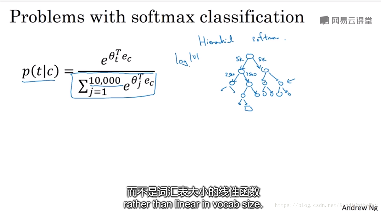
在文献中你会看到的方法是使用一个分级（hierarchical）的softmax分类器，意思就是说不是一下子就确定到底是属于10,000类中的哪一类。想象如果你有一个分类器，它告诉你目标词是在词汇表的前5000个中还是在词汇表的后5000个词中，假如这个二分类器告诉你这个词在前5000个词中（上图编号2所示），然后第二个分类器会告诉你这个词在词汇表的前2500个词中，或者在词汇表的第二组2500个词中，诸如此类，直到最终你找到一个词准确所在的分类器，那么就是这棵树的一个叶子节点。像这样有一个树形的分类器，意味着树上内部的每一个节点都可以是一个二分类器，比如逻辑回归分类器，所以你不需要再为单次分类，对词汇表中所有的10,000个词求和了。实际上用这样的分类树，计算成本与词汇表大小的对数成正比，而不是词汇表大小的线性函数，这个就叫做分级softmax分类器。

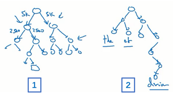
我要提一下，在实践中分级softmax分类器不会使用一棵完美平衡的分类树或者说一棵左边和右边分支的词数相同的对称树（上图编号1所示的分类树）。实际上，分级的softmax分类器会被构造成常用词在顶部，然而不常用的词像durian会在树的更深处（上图编号2所示的分类树），因为你想更常见的词会更频繁，所以你可能只需要少量检索就可以获得常用单词像the和of。然而你更少见到的词比如durian就更合适在树的较深处，因为你一般不需要到那样的深处，所以有不同的经验法则可以帮助构造分类树形成分级softmax分类器。

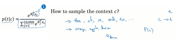
那就是怎么对上下文c进行采样，一旦你对上下文c进行采样，那么目标词t就会在上下文c的正负10个词距内进行采样。但是你要如何选择上下文c？一种选择是你可以就对语料库均匀且随机地采样，如果你那么做，你会发现有一些词，像the、of、a、and、to诸如此类是出现得相当频繁的，于是你那么做的话，你会发现你的上下文到目标词的映射会相当频繁地得到这些种类的词，但是其他词，像orange、apple或durian就不会那么频繁地出现了。你可能不会想要你的训练集都是这些出现得很频繁的词，因为这会导致你花大部分的力气来更新这些频繁出现的单词的$e_c$（上图编号1所示），但你想要的是花时间来更新像durian这些更少出现的词的嵌入，即$e_{durian}$。实际上$p(c)$词的分布并不是单纯的在训练集语料库上均匀且随机的采样得到的，而是采用了不同的分级来平衡更常见的词和不那么常见的词。

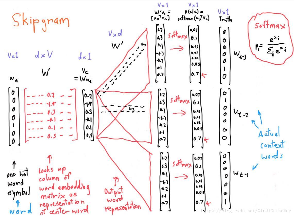
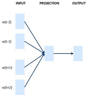
总结下：CBOW是从原始语句推测目标字词；而Skip-Gram正好相反，是从目标字词推测出原始语句。CBOW对小型数据库比较合适，而Skip-Gram在大型语料中表现更好。 （下图左边为CBOW，右边为Skip-Gram）

Negative sampling

In this video, you’ll see a modified learning problem called negative sampling that allows you to do something similar to the Skip-Gram model you saw just now, but with a much more efficient learning algorithm.

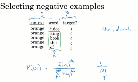
And the problem is, given a pair of words like orange and juice, we're going to predict, is this a context-target pair?

So in this example, orange juice was a positive example. And how about orange and king? Well, that’s a negative example, so I’m going to write 0 for the target.

• So in this case, we have “orange” and “juice” and we’ll associate that with a label of 1, so just put words in the middle. And then having generated a positive example. Sample a context word, look around a window of say, plus-minus ten words and pick a target word. So that’s how you generate the first row of this table with "orange", "juice", 1.

• And then to generate a negative example, you’re going to take the same context word and then just pick a word at random from the dictionary.

  • So in this case, I chose the word “king” at random and we will label that as 0. And then let’s take orange and let’s pick another random word from the dictionary.
  • Under the assumption that if we pick a random word, it probably won’t be associated with the word orange, so orange, book, 0.
  • And let’s pick a few others, orange, maybe just by chance, we’ll pick the 0 “and” then “orange”. And then “orange”, and maybe just by chance, we’ll pick the word of “and” we’ll put a 0 there.
  • And notice that all of these are labeled as 0 even though the word of actually appears next to orange as well.

So to summarize, the way we generated this data set is, we’ll pick a context word and then pick a target word and that is the first row of this table. That gives us a positive example. So context, target, and then give that a label of 1.

And then what we’ll do is for some number of times say, k times, we’re going to take the same context word and then pick random words from the dictionary, king, book, the, of, whatever comes out at random from the dictionary and label all those 0, and those will be our negative examples.

And it’s okay if just by chance, one of those words we picked at random from the dictionary happens to appear in the window, in a plus-minus ten word window say, next to the context word, orange.

Then we’re going to create a supervised learning problem where the learning algorithm inputs x, inputs this pair of words, and it has to predict the target label to predict the output y.

So the problem is really given a pair of words like orange and juice, do you think they appear together? Do you think I got these two words by sampling two words close to each other? It's really to try to distinguish between these two types of distributions from which you might sample a pair of words. So this is how you generate the training set.

How do you choose k
k is 5 to 20 for smaller data sets.
And if you have a very large data set, then chose k to be smaller.
So k equals 2 to 5 for larger data sets, and large values of k for smaller data sets.

$$P(y=1|c,t)=\sigma(\theta_t^Te_c)$$
The parameters are similar as before, you have one parameter vector $\theta_t$ for each possible target word. And a separate parameter vector, really the embedding vector $e_c$, for each possible context word. And we’re going to use this formula to estimate the probability that y is equal to 1.

So if you have k examples here, then you can think of this as having a k to 1 ratio of negative to positive examples. So for every positive examples, you have k negative examples with which to train this logistic regression-like model.

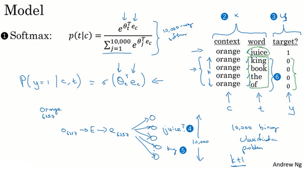
我们把这个画成一个神经网络，如果输入词是orange，即词6257，你要做的就是输入one-hot向量，再传递给$E$，通过两者相乘获得嵌入向量$e_{6257}$，你就得到了10,000个可能的逻辑回归分类问题，其中一个（上图编号4所示）将会是用来判断目标词是否是juice的分类器，还有其他的词，比如说可能下面的某个分类器（上图编号5所示）是用来预测king是否是目标词，诸如此类，预测词汇表中这些可能的单词。把这些看作10,000个二分类逻辑回归分类器，但并不是每次迭代都训练全部10,000个，我们只训练其中的5个，我们要训练对应真正目标词那一个分类器，再训练4个随机选取的负样本，这就是$K=4$的情况。所以不使用一个巨大的10,000维度的softmax，因为计算成本很高，而是把它转变为10,000个二分类问题，每个都很容易计算，每次迭代我们要做的只是训练它们其中的5个，一般而言就是$K+1$个，其中$K$个负样本和1个正样本。这也是为什么这个算法计算成本更低，因为只需更新$K+1$个逻辑单元，$K+1$个二分类问题，相对而言每次迭代的成本比更新10,000维的softmax分类器成本低。

这个技巧就叫负采样。因为你做的是，你有一个正样本词orange和juice，然后你会特意生成一系列负样本，这些（上图编号6所示）是负样本，所以叫负采样，即用这4个负样本训练，4个额外的二分类器，在每次迭代中你选择4个不同的随机的负样本词去训练你的算法。

这个算法有一个重要的细节就是如何选取负样本，即在选取了上下文词orange之后，你如何对这些词进行采样生成负样本？

一个办法是对中间的这些词进行采样，即候选的目标词，你可以根据其在语料中的经验频率进行采样，就是通过词出现的频率对其进行采样。但问题是这会导致你在like、the、of、and诸如此类的词上有很高的频率。另一个极端就是用1除以词汇表总词数，即$\frac{1}{\left|v\right|}$，均匀且随机地抽取负样本，这对于英文单词的分布是非常没有代表性的。

所以论文的作者Mikolov等人根据经验，他们发现这个经验值的效果最好，它位于这两个极端的采样方法之间，既不用经验频率，也就是实际观察到的英文文本的分布，也不用均匀分布，他们采用以下方式：

$P\left( w_{i} \right) = \frac{f\left( w_{i} \right)^{\frac{3}{4}}}{\sum_{j = 1}^{10,000}{f\left( w_{j} \right)^{\frac{3}{4}}}}$

进行采样，所以如果$f(w_{i})$是观测到的在语料库中的某个英文词的词频，通过$\frac{3}{4}$次方的计算，使其处于完全独立的分布和训练集的观测分布两个极端之间。我并不确定这是否有理论证明，但是很多研究者现在使用这个方法，似乎也效果不错。