数据分析–用R语言预测离职(下)
接上一篇~
接下来我们探索离职和其他分类变量的关系~
> library(scales)
> k1 <- ggplot(attr.df, aes(x=Gender,fill=Attrition))+
+   geom_bar(position = "fill")+
+   labs(y="Percentage")+scale_y_continuous(labels = percent)
> k2 <- ggplot(attr.df, aes(x=BusinessTravel,fill=Attrition))+
+   geom_bar(position = "fill")+
+   labs(y="Percentage")+scale_y_continuous(labels = percent)
> k3 <- ggplot(attr.df, aes(x=Department,fill=Attrition))+
+   geom_bar(position = "fill")+
+   labs(y="Percentage")+scale_y_continuous(labels = percent)
> k4 <- ggplot(attr.df, aes(x=EducationField,fill=Attrition))+
+   geom_bar(position = "fill")+
+   labs(y="Percentage")+scale_y_continuous(labels = percent)
> k5 <- ggplot(attr.df, aes(x=MaritalStatus,fill=Attrition))+
+   geom_bar(position = "fill")+
+   labs(y="Percentage")+scale_y_continuous(labels = percent)
> k6 <- ggplot(attr.df, aes(x=OverTime,fill=Attrition))+
+   geom_bar(position = "fill")+
+   labs(y="Percentage")+scale_y_continuous(labels = percent)
> k7 <- ggplot(attr.df, aes(x=JobLevel,fill=Attrition))+
+   geom_bar(position = "fill")+
+   labs(y="Percentage")+scale_y_continuous(labels = percent)
> k8 <- ggplot(attr.df, aes(x=JobSatisfaction,fill=Attrition))+
+   geom_bar(position = "fill")+
+   labs(y="Percentage")+scale_y_continuous(labels = percent)
> k9 <- ggplot(attr.df, aes(x=PerformanceRating,fill=Attrition))+
+   geom_bar(position = "fill")+
+   labs(y="Percentage")+scale_y_continuous(labels = percent)
> k10 <- ggplot(attr.df, aes(x=RelationshipSatisfaction,fill=Attrition))+
+   geom_bar(position = "fill")+
+   labs(y="Percentage")+scale_y_continuous(labels = percent)
> k11 <- ggplot(attr.df, aes(x=WorkLifeBalance,fill=Attrition))+
+   geom_bar(position = "fill")+
+   labs(y="Percentage")+scale_y_continuous(labels = percent)
> k12 <- ggplot(attr.df, aes(x=JobInvolvement,fill=Attrition))+
+   geom_bar(position = "fill")+
+   labs(y="Percentage")+scale_y_continuous(labels = percent)
> grid.arrange(k1,k2,k3,k4,k5,k6,k7,k8,k9,k10,k11,k12, ncol = 3, nrow = 4)
输出结果如图所示:
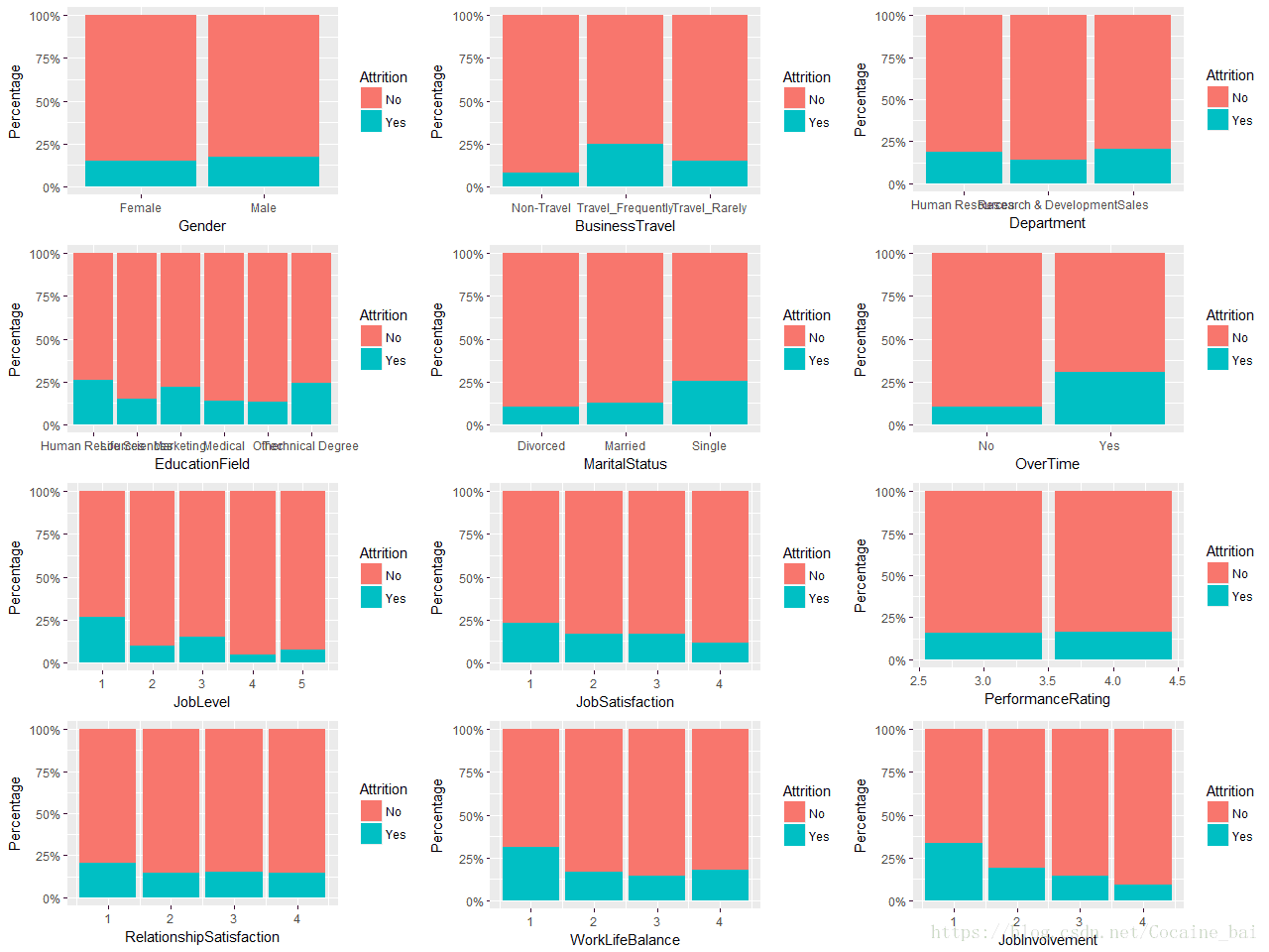
从这几幅图可以看出以下几点:
1.离职的人和性别上面没有多大的差异;
2.出差频繁的人离职的概率要大;
3.单身的人离职的概率要大;
4.从工作满意度,工作投入,人际交往,生活与工作的平衡来看,满意度低的人离职概率偏高;
5.很明显的加班人的离职概率偏高
我们再来看一下工作投入与回报的关系:
> ggplot(attr.df,aes(x=JobInvolvement, y=MonthlyIncome, group=JobInvolvement))+
+   geom_boxplot(aes(fill=factor(JobInvolvement)),alpha=0.7)+
+   theme(legend.position = "none",plot.title = element_text(hjust=0.5))+
+   facet_grid(~Attrition)+ggtitle("Attrition")
输出下图:
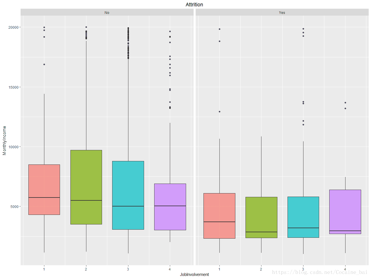
这是一个非常有意思的结果,对于收入高或低,这不能准确说明收入低就是员工流失的原因,
但这里我们可以发现,投入与回报差异较大的,越容易流失,因此企业更需要关注那些投入多但回报少的员工,
这类员工也许不是不努力,而是没有掌握正确的工作方式,应当给予更大的帮助,例如培训,工作指导等;
薪资往往是回报的其中一种。
数据建模
在开始建模之前我们要处理一下数据,缩写一些变量名称和删除不必要的列
# 缩写变量名称
> levels(attr.df$JobRole) <- c("HC","HR","Lab","Man","MDir","RsD","RsSci","SlEx","SlRep")
> levels(attr.df$EducationField) <- c("HR","LS","MRK","MED","NA","TD")

# 删除不必要的列
> attr.df.new <- attr.df[c(-9,-10,-22,-27)]
创建训练集和测试集:
> set.seed(3535)
> n <- nrow(attr.df.new)
> rnd <- sample(n, n*.70)
> train <- attr.df.new[rnd,]
> test <- attr.df.new[-rnd,]
建立决策树模型:
> library(rpart)
> dtree <- rpart(Attrition ~., data = train)
> preds <- predict(dtree, test, type = "class")
> library(pROC)
> rocv <- roc(as.numeric(test$Attrition), as.numeric(preds))
> rocv$auc
Area under the curve: 0.6359
> prop.table(table(test$Attrition, preds, dnn = c("Actual", "Predicted")),1)
      Predicted
Actual         No        Yes
   No  0.98153034 0.01846966
   Yes 0.70967742 0.29032258
AUC(曲线下面积)为0.6359,比较低;灵敏度(查全率)为0.2903,也比较低,
如果用这个模型来直接预测,也许不会得到什么结果,但决策树确实是一个有用的工具,该模型易于理解,我们可以绘制决策树图来看看是否有所发现。
> dtreepr <- prune(dtree, cp=0.018)
> predspr <- predict(dtreepr, test, type="class")
> rocvpr <- roc(as.numeric(test$Attrition), as.numeric(predspr))
> rocvpr$auc
Area under the curve: 0.6589
修建之后的决策树 AUC(曲线下面积)为0.67,没有增加多少精准度
我们来画一下决策树图:
> library(rpart.plot)
> rpart.plot(dtreepr,
+            type=4,
+            extra = 104,
+            tweak = 0.9,
+            fallen.leaves = F,
+            cex = 0.7)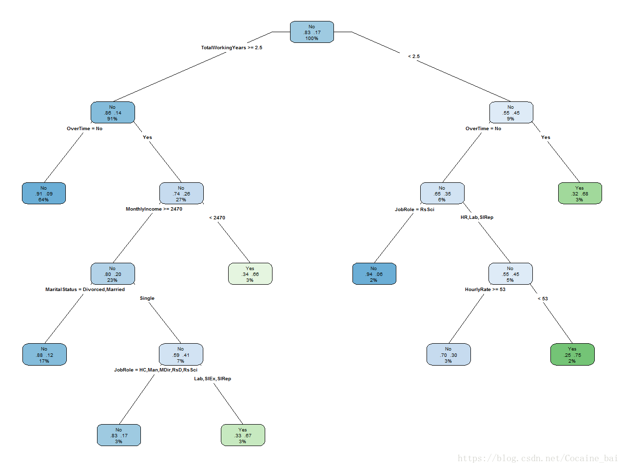
还是可以看出,加班,收入是主要的因素,由于AUC值低于0.75,所以我们要增加模型来提升精准度
使用随机森林和GBM建模
> set.seed(2324)
> library(randomForest)
> fit.forest <- randomForest(Attrition~., data = train)
> rfpreds <- predict(fit.forest, test,type = "class")
> rocf <- roc(as.numeric(test$Attrition), as.numeric(rfpreds))
> rocf$auc
Area under the curve: 0.5874
AUC曲下面积为0.5874,
> set.seed(3333)
> library(gbm)
> library(caret)
> ctrl <- trainControl(method = "cv",
+                      number = 10,
+                      summaryFunction = twoClassSummary,
+                      classProbs = T)
> gbmfit <- train(Attrition ~.,
+                 data = train,
+                 method = "gbm",
+                 verbose = FALSE,
+                 metric = "ROC",
+                 trControl = ctrl)
>
> gbmpreds <- predict(gbmfit, test)
> rocgbm <- roc(as.numeric(test$Attrition), as.numeric(gbmpreds))
> rocgbm$auc
Area under the curve: 0.6493
AUC面积为0.6493,效果依然不是很理想。。。
通过加权、上下采样等方式优化GBM模型
> #设置与前面GBM建模控制器一直的种子
> ctrl$seeds <- gbmfit$control$seeds
>
> # 加权GBM
> # 设置权重参数,提高离开群体的样本权重,平衡样本
> model_weights <- ifelse(train$Attrition == "No",
+                         (1/table(train$Attrition)[1]),
+                         (1/table(train$Attrition)[2]))
> weightedfit <- train(Attrition ~ .,
+                      data = train,
+                      method = "gbm",
+                      verbose = FALSE,
+                      weights = model_weights,
+                      metric = "ROC",
+                      trControl = ctrl)
> weightedpreds <- predict(weightedfit, test)
> rocweight <- roc(as.numeric(test$Attrition), as.numeric(weightedpreds))
> rocweight$auc
Area under the curve: 0.7732
>
> # UP-sampling 向上采样
> ctrl$sampling <- "up"
> set.seed(3433)
> upfit <- train(Attrition ~.,
+                data = train,
+                method = "gbm",
+                verbose = FALSE,
+                metric = "ROC",
+                trControl = ctrl)
>
> uppreds <- predict(upfit, test)
> rocup <- roc(as.numeric(test$Attrition), as.numeric(uppreds))
> rocup$auc
Area under the curve: 0.7345
>
> # DOWN-sampling 向下采样
> ctrl$sampling <- "down"
> set.seed(3433)
> downfit <- train(Attrition ~.,
+                  data = train,
+                  method = "gbm",
+                  verbose = FALSE,
+                  metric = "ROC",
+                  trControl = ctrl)
>
> downpreds <- predict(downfit, test)
> rocdown <- roc(as.numeric(test$Attrition), as.numeric(downpreds))
> rocdown$auc
Area under the curve: 0.7226
结果中,weightedfit 模型表现最好,AUC大于0.75,至此,模型建立完毕~
列出模型中的变量重要性列表:
> varImp(weightedfit)
gbm variable importance

  only 20 most important variables shown (out of 44)

                                 Overall
MonthlyIncome                    100.000
OverTimeYes                       86.478
Age                               73.359
StockOptionLevel                  73.139
DailyRate                         42.851
NumCompaniesWorked                38.342
DepartmentResearch & Development  37.816
JobInvolvement                    35.679
EnvironmentSatisfaction           32.876
BusinessTravelTravel_Frequently   32.205
YearsAtCompany                    27.809
YearsWithCurrManager              25.117
TotalWorkingYears                 23.648
RelationshipSatisfaction          23.562
JobSatisfaction                   23.345
DistanceFromHome                  21.509
PercentSalaryHike                 16.121
JobLevel                          11.765
WorkLifeBalance                   11.203
TrainingTimesLastYear              8.929
影响员工流失的前5个因素是:
月收入
经常加班
年龄
股权
任职过的公司数