Python数据分析基础工具 02 matplotlib 基本使用

版权声明：本文为博主原创文章，未经博主允许不得转载。 https://blog.csdn.net/lihaogn/article/details/81837117

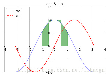
1）基本线图绘制

import matplotlib.pyplot as plt
import numpy as np

x=np.linspace(-np.pi,np.pi,256,endpoint=True)
c,s=np.cos(x),np.sin(x)
# 根据x，y绘制图像
plt.plot(x,c,color="blue",linewidth=1.0,linestyle="-",label="cos",alpha=0.5)
plt.plot(x,s,"r--",label="sin")
# 设置图的名称
plt.title("cos & sin")
# 获取图像编辑器
ax=plt.gca()
# 设置右边界和上边界
ax.spines["right"].set_color("none")
ax.spines["top"].set_color("none")
# 设置坐标轴位置
ax.spines["left"].set_position(("data",0))
ax.spines["bottom"].set_position(("data",0))
# 打印图例
plt.legend(loc="upper left")
# 打印网络线
plt.grid()
# 设置坐标轴显示范围
plt.axis([-4,4,-1,1.5])
# 指定位置填充，当abs(x)<0.5时，从1开始填充到c；当abs(x)>0.5时，从0开始填充到c
plt.fill_between(x,np.abs(x)<0.5,c,c>0.5,color="green",alpha=0.5)
plt.show()

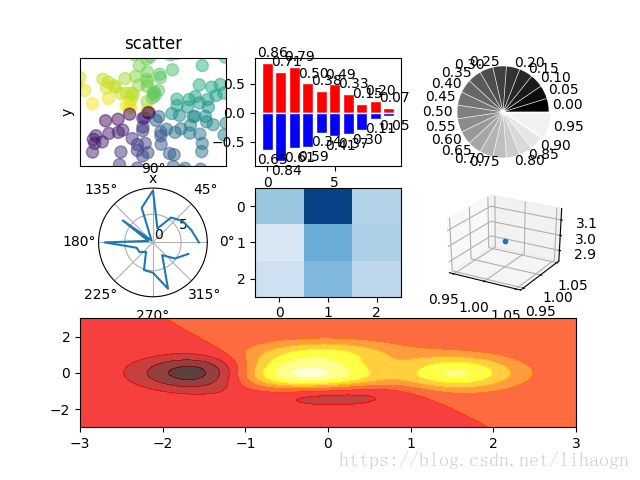
2）子图与多种图形绘制

import numpy as np
import matplotlib.pyplot as plt

fig = plt.figure()

# *** 绘制散点图

# 3行3列的第一个图
ax = fig.add_subplot(3, 3, 1)

n = 128
xx = np.random.normal(0, 1, n)
yy = np.random.normal(0, 1, n)

# 用于上色
tt = np.arctan2(yy, xx)
# 指定显示范围
# plt.axes([0.025,0.025,0.95,0.95])
# 绘制散点图，s表示大小，c表示color
# plt.scatter(xx,yy,s=75,c=tt,alpha=0.5)
ax.scatter(xx, yy, s=75, c=tt, alpha=0.5)
# x范围
plt.xlim(-1.5, 1.5), plt.xticks([])
# y范围
plt.ylim(-1.5, 1.5), plt.yticks([])
plt.axis()
plt.title("scatter")
plt.xlabel("x")
plt.ylabel("y")

# *** 绘制柱状图
fig.add_subplot(3, 3, 2)
n = 10
xx = np.arange(n)
y1 = (1 - xx / float(n)) * np.random.uniform(0.5, 1.0, n)
y2 = (1 - xx / float(n)) * np.random.uniform(0.5, 1.0, n)

# +,-表示绘图位置
plt.bar(xx, +y1, facecolor='r', edgecolor='white')
plt.bar(xx, -y2, facecolor='blue', edgecolor='white')

for x, y in zip(xx, y1):
    plt.text(x + 0.4, y + 0.05, '%.2f' % y, ha='center', va='bottom')
for x, y in zip(xx, y2):
    plt.text(x + 0.4, -y - 0.05, '%.2f' % y, ha='center', va='top')

# *** 绘制饼图

fig.add_subplot(3, 3, 3)

n = 20
z = np.ones(n)
z[-1] *= 2

# explode代表离中心的距离
plt.pie(z, explode=z * 0.05, colors=['%f' % (i / float(n)) for i in range(n)],
        labels=['%.2f' % (i / float(n)) for i in range(n)])
# 绘制成正圆形
plt.gca().set_aspect('equal')
plt.xticks([]), plt.yticks([])

# 绘制极坐标
fig.add_subplot(334, polar=True)
n = 20
theta = np.arange(0.0, 2 * np.pi, 2 * np.pi / n)
radii = 10 * np.random.rand(n)
# plt.plot(theta, radii)
plt.polar(theta, radii)

# 绘制热图
fig.add_subplot(335)
from matplotlib import cm

data = np.random.rand(3, 3)
cmap = cm.Blues
map = plt.imshow(data, interpolation='nearest', cmap=cmap, aspect='auto', vmin=0, vmax=1)

# 绘制3d图
from mpl_toolkits.mplot3d import Axes3D

ax = fig.add_subplot(336, projection="3d")
ax.scatter(1, 1, 3, s=10)

# 绘制热力图
fig.add_subplot(313)


def f(x, y):
    return (1 - x / 2 + x ** 5 + y ** 3) * np.exp(-x ** 2 - y ** 2)


n = 256
x = np.linspace(-3, 3, n)
y = np.linspace(-3, 3, n)
xx, yy = np.meshgrid(x, y)
plt.contourf(xx, yy, f(xx, yy), 8, alpha=.75, cmap=plt.cm.hot)

plt.show()