Python数据分析（8）matplotlib库的使用：基本图像类型（直方图，条形图，饼图）

#coding=gbk
import matplotlib.pyplot as plt
import numpy as np
#图像的基本 类型
#1.线性图
x=np.arange(-2*np.pi,2*np.pi,0.01)
y1=np.sin(3*x)/x
y2=np.sin(2*x)/x
y3=np.sin(4*x)/x
plt.plot(x,y1)
plt.plot(x,y2,'k--',linewidth=2)    #调整线宽，k为黑色的
plt.plot(x,y3,'m--')
plt.title('线性表',fontproperties='SimHei',fontsize=25,color='red')
plt.show()      #画多条线时，会自动调整不同的颜色

#横坐标修改为pi
x=np.arange(-2*np.pi,2*np.pi,0.01)
y1=np.sin(3*x)/x
y2=np.sin(2*x)/x
y3=np.sin(4*x)/x
plt.plot(x,y1)
plt.plot(x,y2,'k--',linewidth=2)    #调整线宽，k为黑色的
plt.plot(x,y3,'m--')
plt.title('线性表',fontproperties='SimHei',fontsize=15,color='red')
plt.xticks([-2*np.pi,-np.pi,0,np.pi, 2*np.pi],
           [r'$-2\pi$',r'$-\pi$',r'$0$',r'$\pi$',r'$2\pi$'])#修改横坐标的数字
plt.yticks([-1,0,+1,+2,+3],[r'$-1$',r'$0$',r'$+1$',r'$+2$',r'$+3$'])
plt.show()

#将pandas库的DataFrame对象画图
import pandas as pd
data={'series1':[1,2,4,8,13],
      'series2':[2,5,8,12,16],
      'series3':[4,6,2,7,9]}
df=pd.DataFrame(data)
x=np.arange(5)
plt.axis([0,5,0,17])    #设置横坐标，纵轴长度
plt.plot(x,df)
plt.legend(df,loc=0)    #此处使用df 和 data 都可以
plt.show()

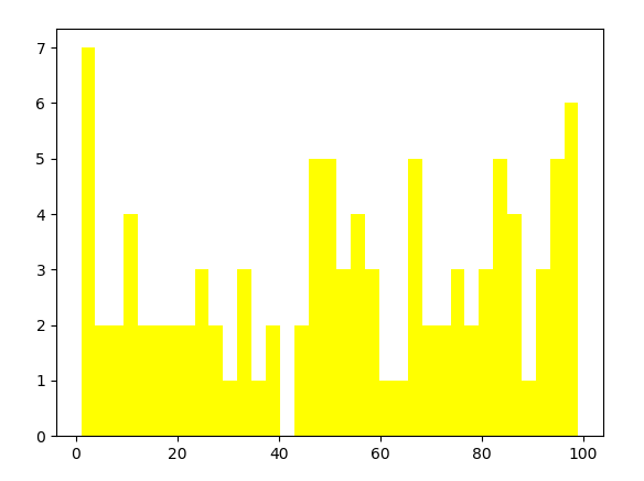
#2直方图
np.random.seed(123) #设定随机种子
p=np.random.randint(0,100,100)
plt.hist(p,35,color='yellow')  #分成35个区间
plt.show()

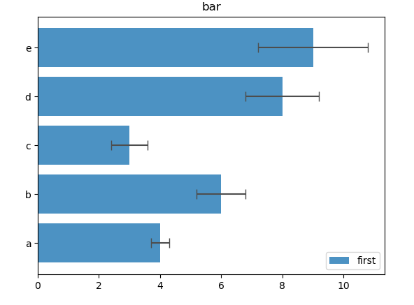
#3条状图
# 带误差线的条状图
 x=np.arange(5)
 y=[4,6,3,8,9]
 std=[0.3,0.8,0.6,1.2,1.8]   #设为标准差
 plt.title('bar')
 plt.xticks(x,['a','b','c','d','e'])
 plt.bar(x,y,yerr=std,alpha=0.8,label='first',error_kw={'ecolor':'0.3','capsize':5})
 #    ecolor表示为黑线的透明度，capsize为横线的长度
 plt.legend(loc=2)
 plt.show()

颜色参数：

#水平条状图
#改变参数 yticks 和 xerr
x=np.arange(5)
y=[4,6,3,8,9]
std=[0.3,0.8,0.6,1.2,1.8]   #设为标准差
plt.title('bar')
plt.yticks(x,['a','b','c','d','e'])
plt.barh(x,y,xerr=std,alpha=0.8,label='first',error_kw={'ecolor':'0.3','capsize':5})
#    ecolor表示为黑线的透明度，capsize为横线的长度
plt.legend(loc=4)
plt.show()

#多序列条状图
x=np.arange(5)
y1=[4,6,3,8,9]
y2=[2,3,6,7,10]
y3=[1,6,3,9,15]
plt.title('bar')
bw=0.3      #间隔为bw
plt.xticks(x+bw,['a','b','c','d','e'])
plt.bar(x,y1,bw,color='b')
plt.bar(x+bw,y2,bw,color='g')
plt.bar(x+2*bw,y3,bw,color='r')
plt.show()

#为DataFrame数据结构画bar图
data={'series1':[1,2,4,8,13],
      'series2':[2,5,8,12,16],
      'series3':[4,6,2,7,9]}
df=pd.DataFrame(data)
df.plot(kind='bar')
plt.show()

#多序列堆积图
x=np.arange(5)
y1=np.array([4,6,3,8,9])    #需要定义为array数组
y2=np.array([2,3,6,7,10])
y3=np.array([1,6,3,9,5])
plt.xticks(x+0.2,['a','b','c','d','e'])
plt.axis([0,6,0,25])
plt.bar(x,y1,color='b')
plt.bar(x,y2,color='g',bottom=y1)   #以y1为低，bottom
plt.bar(x,y3,color='r',bottom=(y1+y2))
plt.show()

#为dataFrame 数据结构画堆积图
data={'series1':[1,2,4,8,13],
      'series2':[2,5,8,12,16],
      'series3':[4,6,2,7,9]}
df=pd.DataFrame(data)
df.plot(kind='bar',stacked=True)
plt.show()

#3饼图
values=[12,24,45,60,12]
labels=['book','pen','pencil','notebook','desk']
color=['red','yellow','black','blue','green']
explode=[0.3,0,0,0,0]   #脱离圆的程度，0为为脱离，1为完全脱离
plt.pie(values,labels=labels,colors=color,explode=explode,startangle=90,
        autopct='%1.1f% %',shadow=True)  #autopct表示显示每个标签的百分比
plt.axis('equal')
plt.show()

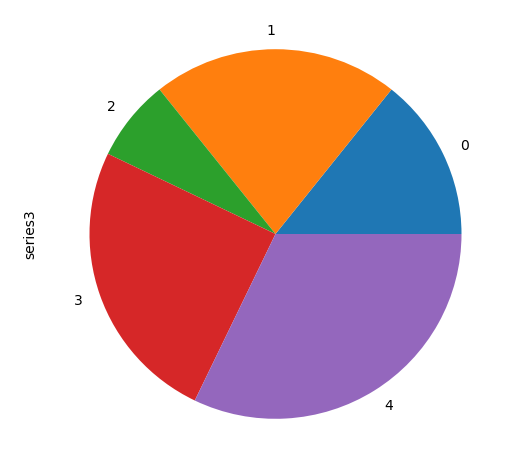
#为dataFrame 数据结构画饼图
data={'series1':[1,2,4,8,13],
      'series2':[2,5,8,12,16],
      'series3':[4,6,2,7,9]}
df=pd.DataFrame(data)
df['series3'].plot(kind='pie',figsize=(6,6))
plt.show()