机器学习入门 03 线性回归法（Linear Regression）

1 简单线性回归

1.1 介绍

1）特点：

• 样本特征只有一个
• 解决回归问题
• 思想简单，实现容易
• 许多强大的非线性模型的基础
• 结果有很好的解释性

1.2 思想、公式

1.2.1 思想

寻找出一条直线，最大程度的“拟合”样本特征和样本输出标记之间的关系。

通过分析问题，确定问题的损失函数（loss function）或效用函数（utility function）；

通过最优化损失函数（min）或效用函数（max），获得机器学习的模型。

近乎所有参数学习算法都是这样的套路。

1.2.2 公式

线性关系：$y=ax+b$

对应关系：${ y }^{ (i) }=a{ x }^{ (i) }+b$，${ \overset { \wedge }{ y } }^{ (i) }=a{ x }^{ (i) }+b$；

• ${ x }^{ (i) }$为样本点的值
• ${ y }^{ (i) }$为样本对应的真实值
• ${ \overset { \wedge }{ y } }^{ (i) }$为预测值

表达差距（损失函数）：${ \left( { y }^{ (i) }-{ \overset { \wedge }{ y } }^{ (i) } \right) }^{ 2 }$

考虑所有的样本的差距：$\sum _{ i=1 }^{ m }{ { \left( { y }^{ (i) }-{ \overset { \wedge }{ y } }^{ (i) } \right) }^{ 2 } } =\sum _{ i=1 }^{ m }{ { \left( { y }^{ (i) }-a{ x }^{ (i) }-b \right) }^{ 2 } }$

简单线性回归的目标：找到 a，b 使得上式的值最小。

1.2.3 求出 a，b

目标函数：$f=\sum _{ i=1 }^{ m }{ { \left( { y }^{ (i) }-a{ x }^{ (i) }-b \right) }^{ 2 } }$

1）分别对 a，b 求一阶导，令其导函数为0，求解 a，b

$\frac { \sigma f }{ \sigma b } =0\\ \sum _{ i=1 }^{ m }{ 2\left( { y }^{ (i) }-a{ x }^{ (i) }-b \right) \left( -1 \right) =0 } \\ \sum _{ i=1 }^{ m }{ \left( { y }^{ (i) }-a{ x }^{ (i) }-b \right) =0 } \\ \sum _{ i=1 }^{ m }{ { y }^{ (i) } } -\sum _{ i=1 }^{ m }{ a{ x }^{ (i) } } -\sum _{ i=1 }^{ m }{ b } =0\\ \sum _{ i=1 }^{ m }{ { y }^{ (i) } } -\sum _{ i=1 }^{ m }{ a{ x }^{ (i) } } -mb=0\\ mb=\sum _{ i=1 }^{ m }{ { y }^{ (i) } } -\sum _{ i=1 }^{ m }{ a{ x }^{ (i) } } \\ b=\overline { y } -a\overline { x }$

$\frac { \sigma f }{ \sigma a } =0\\ \sum _{ i=1 }^{ m }{ 2\left( { y }^{ (i) }-a{ x }^{ (i) }-b \right) \left( -{ x }^{ (i) } \right) =0 } \\ \sum _{ i=1 }^{ m }{ \left( { y }^{ (i) }-a{ x }^{ (i) }-b \right) ({ x }^{ (i) })=0 } \\ \sum _{ i=1 }^{ m }{ \left( { y }^{ (i) }-a{ x }^{ (i) }-\overline { y } +a\overline { x } \right) ({ x }^{ (i) })=0 } \\ \sum _{ i=1 }^{ m }{ \left( { { x }^{ (i) }y }^{ (i) }-a{ { (x }^{ (i) } })^{ 2 }-{ x }^{ (i) }\overline { y } +a\overline { x } { x }^{ (i) } \right) =0 } \\ \sum _{ i=1 }^{ m }{ ({ { x }^{ (i) }y }^{ (i) }-{ x }^{ (i) }\overline { y } ) } -\sum _{ i=1 }^{ m }{ (a{ { (x }^{ (i) } })^{ 2 }-a\overline { x } { x }^{ (i) }) } =0\\ \sum _{ i=1 }^{ m }{ ({ { x }^{ (i) }y }^{ (i) }-{ x }^{ (i) }\overline { y } ) } -a\sum _{ i=1 }^{ m }{ ({ { (x }^{ (i) } })^{ 2 }-\overline { x } { x }^{ (i) }) } =0\\ a=\frac { \sum _{ i=1 }^{ m }{ ({ { x }^{ (i) }y }^{ (i) }-{ x }^{ (i) }\overline { y } ) } }{ \sum _{ i=1 }^{ m }{ ({ { (x }^{ (i) } })^{ 2 }-\overline { x } { x }^{ (i) }) } } \\ \because \sum { { x }^{ (i) }\overline { y } } =\overline { y } \sum { { x }^{ (i) } } =m\overline { x } \overline { y } =\sum { \overline { x } \overline { y } } =\overline { x } \sum { { y }^{ (i) } } =\sum { \overline { x } { y }^{ (i) } } \\ \therefore \quad a=\frac { \sum _{ i=1 }^{ m }{ ({ { x }^{ (i) }y }^{ (i) }-{ x }^{ (i) }\overline { y } -\overline { x } { y }^{ (i) }+\overline { x } \overline { y } ) } }{ \sum _{ i=1 }^{ m }{ ({ { (x }^{ (i) } })^{ 2 }-\overline { x } { x }^{ (i) }-\overline { x } { x }^{ (i) }+{ (\overline { x } ) }^{ 2 }) } } =\frac { \sum _{ i=1 }^{ m }{ ({ x }^{ (i) }-\overline { x } )({ y }^{ (i) }-\overline { y } ) } }{ \sum _{ i=1 }^{ m }{ { ({ x }^{ (i) }-\overline { x } ) }^{ 2 } } }$

2）a与b的值
$a=\frac { \sum _{ i=1 }^{ m }{ ({ { x }^{ (i) }y }^{ (i) }-{ x }^{ (i) }\overline { y } -\overline { x } { y }^{ (i) }+\overline { x } \overline { y } ) } }{ \sum _{ i=1 }^{ m }{ ({ { (x }^{ (i) } })^{ 2 }-\overline { x } { x }^{ (i) }-\overline { x } { x }^{ (i) }+{ (\overline { x } ) }^{ 2 }) } } =\frac { \sum _{ i=1 }^{ m }{ ({ x }^{ (i) }-\overline { x } )({ y }^{ (i) }-\overline { y } ) } }{ \sum _{ i=1 }^{ m }{ { ({ x }^{ (i) }-\overline { x } ) }^{ 2 } } }$

$b=\overline { y } -a\overline { x }$

2 衡量线性回归算法的指标

2.1 均方误差 MSE（Mean Squared Error）

$f=\frac { 1 }{ m } \sum { { ({ y }_{ test }^{ (i) }-{ \widehat { y } }_{ test }^{ (i) }) }^{ 2 } }$

2.2 均方根误差 RMSE（Root Mean Squared Error）

$f=\sqrt { { MSE }_{ test } } =\sqrt { \frac { 1 }{ m } \sum { { ({ y }_{ test }^{ (i) }-{ \widehat { y } }_{ test }^{ (i) }) }^{ 2 } } }$

2.3 平均绝对误差 MAE（Mean Absolute Error）

$f=\frac { 1 }{ m } \sum { \left| { y }_{ test }^{ (i) }-{ \widehat { y } }_{ test }^{ (i) } \right| }$

2.4 R Squared

${ R }^{ 2 }=1-\frac { { SS }_{ residual } }{ { SS }_{ total } } =1-\frac { \sum _{ i=1 }^{ m }{ { ({ \widehat { y } }^{ (i) }-{ y }^{ (i) }) }^{ 2 } } }{ \sum _{ i=1 }^{ m }{ { (\overline { y } -{ y }^{ (i) }) }^{ 2 } } } \\ \quad =1-\frac { { \sum _{ i=1 }^{ m }{ { ({ \widehat { y } }^{ (i) }-{ y }^{ (i) }) }^{ 2 } } }/{ m } }{ { \sum _{ i=1 }^{ m }{ { (\overline { y } -{ y }^{ (i) }) }^{ 2 } } }/{ m } } =1-\frac { MSE(\widehat { y } ,y) }{ var(y) }$

• ${ SS }_{ residual }$ –> Residual sum of squares
• ${ SS }_{ total }$ –> Total sum of squares
• $var(y)$ –> y的方差

性质：

• ${ R }^{ 2 }$越大越好，当预测模型不犯错误时，${ R }^{ 2 }$=1
• ${ R }^{ 2 }$<=1
• 当预测模型=基准模型时，${ R }^{ 2 }$=0
• 如果${ R }^{ 2 }$<0，则我们的模型还不如基准模型，即意味着我们的数据不存在任何的线性关系。

3 多元线性回归和正规方程解

1）多元线性回归的样本特征有多个。
2）表达式：

• $y={ \theta }_{ 0 }{ x }_{ 0 }+{ \theta }_{ 1 }{ x }_{ 1 }+{ \theta }_{ 2 }{ x }_{ 2 }+\dots +{ \theta }_{ n }{ x }_{ n }，{ x }_{ 0 }\equiv 1$
• ${ \widehat { y } }^{ (i) }={ \theta }_{ 0 }{ x }_{ 0 }^{ (i) }+{ \theta }_{ 1 }{ x }_{ 1 }^{ (i) }+{ \theta }_{ 2 }{ x }_{ 2 }^{ (i) }+\dots { \theta }_{ n }{ x }_{ n }^{ (i) }，{ x }_{ 0 }^{ (i) }\equiv 1$

3）差距表达式：$f=\sum _{ i=1 }^{ m }{ { ({ y }^{ (i) }-{ \widehat { y } }^{ (i) }) }^{ 2 } } ={ (\overrightarrow { y } -\overrightarrow { { x }_{ b } } ) }^{ \intercal }(\overrightarrow { y } -\overrightarrow { { x }_{ b } } )$

4）目标：找到$\overrightarrow { \theta } ={ ({ \theta }_{ 0 },{ \theta }_{ 1 },{ \theta }_{ 2 },\dots ,{ \theta }_{ n },) }^{ \intercal }$，使得上式 $f$ 的值最小。

• $\overrightarrow { { x }_{ b } } =\begin{Bmatrix} 1 & { x }_{ 1 }^{ (1) } & { x }_{ 2 }^{ (1) } & \dots & { x }_{ n }^{ (1) } \\ 1 & { x }_{ 1 }^{ (2) } & { x }_{ 2 }^{ (2) } & \dots & { x }_{ n }^{ (2) } \\ \vdots & \vdots & \vdots & \ddots & \vdots \\ 1 & { x }_{ 1 }^{ (m) } & { x }_{ 2 }^{ (m) } & \dots & { x }_{ n }^{ (m) } \end{Bmatrix}$
• $\overrightarrow { \widehat { y } } =\vec { { x }_{ b } } \vec { \theta }$
• ${ \theta }_{ 0 }$ 为截距（intercept)，${ \theta }_{ 0 }\cdots { \theta }_{ n }$ 为系数（coefficients)。

5）求解，对 $f$ 求导可求出$\vec { \theta }$，即多元线性回归的正规方程解（Normal Equation）

$\vec { \theta } ={ ({ x }_{ b }^{ \intercal }{ x }_{ b }) }^{ -1 }{ x }_{ b }^{ \intercal }y$

此公式特点：

• 问题：时间复杂度高，O(n^3)，优化后O(n^2.4)。
• 优点：不需要进行数据归一化处理。

4 代码

4.1 简单线性回归

1）SimpleLR.py

import numpy as np
from comm_utils.testCapability import r2_score


class SimpleLinearRegression:

    def __init__(self):
        """ 初始化Simple Linear Regression 模型"""
        self.a_ = None
        self.b_ = None

    def fit(self, x_train, y_train):
        """ 根据训练数据集x_train,y_train训练simple LR 模型"""
        assert x_train.ndim == 1, "simple LR can only solve single feature traing data."
        assert len(x_train) == len(y_train), "the size of x_train must be equal to the size of y_train"

        x_mean = np.mean(x_train)
        y_mean = np.mean(y_train)

        # 使用向量的方式计算
        self.a_ = (x_train - x_mean).dot(y_train - y_mean) / (x_train - x_mean).dot(x_train - x_mean)
        self.b_ = y_mean - self.a_ * x_mean

        return self

    def predict(self, x_predict):
        """ 给定待预测数据集x_predict,返回表示x_predict的结果向量"""
        assert x_predict.ndim == 1, "simple LR can only solve single feature traing data."
        assert self.a_ is not None and self.b_ is not None, "must fit before predict."

        return np.array([self._predict(x) for x in x_predict])

    def _predict(self, x_single):
        """ 给定单个待预测数据x，返回x的预测结果值"""
        return self.a_ * x_single + self.b_

    def score(self, x_test, y_test):
        """ 根据测试数据集 x_test 和 y_test 确定当前模型的准确度"""
        y_predict = self.predict(x_test)
        return r2_score(y_test, y_predict)

    def __repr__(self):
        return "simpleLR()"

4.2 多元线性回归

1）LinearRegression.py

import numpy as np
from comm_utils.testCapability import r2_score


class LinearRegression:

    def __init__(self):
        """ 初识化 LR 模型"""
        self.coef_ = None
        self.intercept_ = None
        self._theta = None

    def fit_normal(self, x_train, y_train):
        """ 根据训练数据集x_train,y_train训练LR模型"""
        assert x_train.shape[0] == y_train.shape[0], "the size of x_train must be equal to the size of y_train"

        # 在第一列前添加一列1
        x_b = np.hstack([np.ones((len(x_train), 1)), x_train])
        self._theta = np.linalg.inv(x_b.T.dot(x_b)).dot(x_b.T).dot(y_train)

        self.intercept_ = self._theta[0]
        self.coef_ = self._theta[1:]

        return self

    def predict(self, x_predict):
        """ 给定待预测数据集x_predict,返回表示x_predict的结果向量"""
        assert self.intercept_ is not None and self.coef_ is not None, "must fit before predict."
        assert x_predict.shape[1] == len(self.coef_), "the feature number of x_predict must be equal to x_train"

        x_b = np.hstack([np.ones((len(x_predict), 1)), x_predict])
        return x_b.dot(self._theta)

    def score(self, x_test, y_test):
        """ 根据测试数据集 x_test 和 y_test 确定当前模型的准确度"""
        y_predict = self.predict(x_test)
        return r2_score(y_test, y_predict)

    def __repr__(self):
        return "LinearRegression()"

4.3 测试

1）model_selection.py

import numpy as np


def train_test_split(x, y, test_reaio=0.2, seed=None):
    """ 将数据x和y按照test_ratio分割成x_train,x_test,y_train,y_test"""

    assert x.shape[0] == y.shape[0], "the size of x must be equal to the y"
    assert 0.0 <= test_reaio <= 1.0, "test_ratio must be valid"

    if seed:
        np.random.seed(seed)

    shuffled_indexes = np.random.permutation(len(x))

    test_size = int(len(x) * test_reaio)
    test_indexes = shuffled_indexes[:test_size]
    train_indexes = shuffled_indexes[test_size:]

    x_train = x[train_indexes]
    y_train = y[train_indexes]

    x_test = x[test_indexes]
    y_test = y[test_indexes]

    return x_train, x_test, y_train, y_test

2）testCapability.py

import numpy as np
from math import sqrt


def accuracy_score(y_true, y_predict):
    """ 计算y_true和y_predict之间的准确率"""
    assert len(y_true) == len(y_predict), \
        "the size of y_true must be equal to the size of y_predict"

    return np.sum(y_true == y_predict) / len(y_true)


def mean_squared_error(y_true, y_predict):
    """ 计算y_true和y_predict之间的MSE"""
    assert len(y_true) == len(y_predict), \
        "the size of y_true must be equal to the size of y_predict"

    return np.sum((y_true - y_predict) ** 2) / len(y_true)


def root_mean_squared_error(y_true, y_predict):
    """ 计算y_true和y_predict之间的RMSE"""

    return sqrt(mean_squared_error(y_true, y_predict))


def mean_absolute_error(y_true, y_predict):
    """ 计算y_true和y_predict之间的MAE"""
    assert len(y_true) == len(y_predict), \
        "the size of y_true must be equal to the size of y_predict"

    return np.sum(np.absolute(y_true - y_predict)) / len(y_true)


def r2_score(y_true, y_predict):
    """ 计算y_true和y_predict之间的R Square"""

    return 1 - mean_squared_error(y_true, y_predict) / np.var(y_true)

3）test.py

import matplotlib.pyplot as plt
from sklearn import datasets
from comm_utils.model_selection import train_test_split
import LinearRegression_pro.SimpleLR

# 准备数据，波士顿房产数据
boston = datasets.load_boston()
print(boston.feature_names)
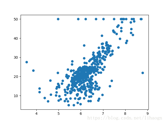
x = boston.data[:, 5]  # 只使用房间数量这个特征
print(x.shape)
y = boston.target
print(y.shape)
# 绘制图
plt.scatter(x, y)
plt.show()

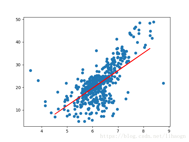
# 去除 y 为50的特殊值
x = x[y < 50.0]
y = y[y < 50.0]

plt.scatter(x, y)


# 使用简单线性回归法

# 1 拆分数据集
x_train, x_test, y_train, y_test = train_test_split(x, y)
# 2 拟合
slr = LinearRegression_pro.SimpleLR.SimpleLinearRegression()
slr.fit(x_train, y_train)
print(slr.score(x_test, y_test))
# 3 绘制出线性关系
plt.plot(x_test, slr.predict(x_test), color="red")
plt.show()

运行结果：

['CRIM' 'ZN' 'INDUS' 'CHAS' 'NOX' 'RM' 'AGE' 'DIS' 'RAD' 'TAX' 'PTRATIO'
 'B' 'LSTAT']
(506,)
(506,)
0.5857523540718015

4）test1.py

from sklearn import datasets
from comm_utils.model_selection import train_test_split
import LinearRegression_pro.LinearRegression

# 准备数据，波士顿房产数据
boston = datasets.load_boston()

x = boston.data
y = boston.target

x = x[y < 50.0]
y = y[y < 50.0]

print(x.shape)
print(y.shape)


# 使用线性回归法

# 1 拆分数据集
x_train, x_test, y_train, y_test = train_test_split(x, y)
# 2 拟合
slr = LinearRegression_pro.LinearRegression.LinearRegression()
slr.fit_normal(x_train, y_train)
# 3 测试性能
print(slr.score(x_test, y_test))

运行结果：

(490, 13)
(490,)
0.7327444560557277

5 总结

• 典型的参数学习，kNN是非参数学习
• 只能解决回归问题
• 对数据有假设：线性
• 对数据具有强解释性