模型评估和验证【1】——过拟合与欠拟合的解决方法

模型评估和验证【1】——过拟合与欠拟合的解决方法

---

1.模型的误差产生的机制

• 误差（Error）：模型预测结果与真实结果之间的差异
• 偏差（bias）：模型的训练误差叫做偏差
• 方差（Variance）：训练误差和测试误差的差异大小叫方差

1.1 欠拟合与过拟合

       欠拟合：在训练数据和未知数据上表现都很差，高偏差

解决方法：

1）添加其他特征项，有时候我们模型出现欠拟合的时候是因为特征项不够导致的，可以添加其他特征项来很好地解决。例如，“组合”、“泛化”、“相关性”三类特征是特征添加的重要手段，无论在什么场景，都可以照葫芦画瓢，总会得到意想不到的效果。除上面的特征之外，“上下文特征”、“平台特征”等等，都可以作为特征添加的首选项。

2）添加多项式特征，这个在机器学习算法里面用的很普遍，例如将线性模型通过添加二次项或者三次项使模型泛化能力更强。例如上面的图片的例子。

3）减少正则化参数，正则化的目的是用来防止过拟合的，但是现在模型出现了欠拟合，则需要减少正则化参数。

     

      过拟合： 在训练数据上表现良好，在未知数据上表现差。高方差

通俗一点地来说过拟合就是模型把数据学习的太彻底，以至于把噪声数据的特征也学习到了，这样就会导致在后期测试的时候不能够很好地识别数据，即不能正确的分类，模型泛化能力太差。例如下面的例子。

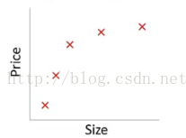
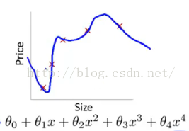
上面左图表示size和prize的关系，我们学习到的模型曲线如右图所示，虽然在训练的时候模型可以很好地匹配数据，但是很显然过度扭曲了曲线，不是真实的size与prize曲线。

解决方法：

1）重新清洗数据，导致过拟合的一个原因也有可能是数据不纯导致的，如果出现了过拟合就需要我们重新清洗数据。

2）增大数据的训练量，还有一个原因就是我们用于训练的数据量太小导致的，训练数据占总数据的比例过小。

3）采用正则化方法。

        正则化方法包括L0正则、L1正则和L2正则，而正则一般是在目标函数之后加上对余的范数。但是在机器学习中一般使用L2正则，下面看具体的原因。

 L1范数是指向量中各个元素绝对值之和，也叫“稀疏规则算子”（Lasso regularization）。

  两者都可以实现稀疏性，既然L0可以实现稀疏，为什么不用L0，而要用L1呢？个人理解一是因为L0范数很难优化求解（NP难问题），二是L1范数是L0范数的最优凸近似， 而且它比L0范数要容易优化求解。所以大家才把目光和万千宠爱转于L1范数。

L2范数是指向量各元素的平方和然后求平方根。可以使得W的每个元素都很小，都接近于0，但与L1范数不同，它不会让它等于0，而是接近于0。L2正则项起到使得参数w变小加剧的效果，但是为什么可以防止过拟合呢？一个通俗的理解便是：更小的参数值w意味着模型的复杂度更低，对训练数据的拟合刚刚好（奥卡姆剃刀），不会过分拟合训练数据，从而使得不会过拟合，以提高模型的泛化能力。还有就是看到有人说L2范数有助于处理 condition number不好的情况下矩阵求逆很困难的问题（具体这儿我也不是太理解）。

4）采用dropout方法。这个方法在神经网络里面很常用。dropout方法是ImageNet中提出的一种方法，通俗一点讲就是dropout方法在训练的时候让神经元以一定的概率不工作。具体看下图：

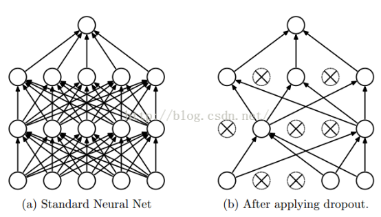
如上图所示，左边a图是没用用dropout方法的标准神经网络，右边b图是在训练过程中使用了dropout方法的神经网络，即在训练时候以一定的概率p来跳过一定的神经元。

其中正则化的方法转至：正则化的理解

1.2 学习曲线诊断模型的偏差和方差

机器学习系统的设计流程

Step1.使用快速但不完美的算法实现；

Step2.画出学习曲线，分析偏差、方差，判断是否需要更多的数据、增加特征量....;

Step3.误差分析:人工检测错误、发现系统短处，来增加特征量以改进系统。

---

学习曲线是什么？

学习曲线就是通过画出不同训练集大小时训练集和交叉验证的准确率，可以看到模型在新数据上的表现，进而来判断模型是否方差偏高或偏差过高，以及增大训练集是否可以减小过拟合。

# 学习曲线诊断偏差和方差问题
%matplotlib inline
import matplotlib.pyplot as plt
from sklearn.learning_curve import learning_curve
 
pipe_lr = Pipeline([('scl', StandardScaler()),
            ('clf', LogisticRegression(penalty='l2', random_state=0))])
 
train_sizes, train_scores, test_scores =\
                learning_curve(estimator=pipe_lr, 
                X=X_train, 
                y=y_train, 
                train_sizes=np.linspace(0.1, 1.0, 10), 
                cv=10,
                n_jobs=1)
 
train_mean = np.mean(train_scores, axis=1)
train_std = np.std(train_scores, axis=1)
test_mean = np.mean(test_scores, axis=1)
test_std = np.std(test_scores, axis=1)
 
plt.plot(train_sizes, train_mean, 
         color='blue', marker='o', 
         markersize=5, label='training accuracy')
 
plt.fill_between(train_sizes, 
                 train_mean + train_std,
                 train_mean - train_std, 
                 alpha=0.15, color='blue')
 
plt.plot(train_sizes, test_mean, 
         color='green', linestyle='--', 
         marker='s', markersize=5, 
         label='validation accuracy')
 
plt.fill_between(train_sizes, 
                 test_mean + test_std,
                 test_mean - test_std, 
                 alpha=0.15, color='green')
 
plt.grid()
plt.xlabel('Number of training samples')
plt.ylabel('Accuracy')
plt.legend(loc='lower right')
plt.ylim([0.8, 1.0])
plt.tight_layout()
# plt.savefig('./figures/learning_curve.png', dpi=300)
plt.show()

注：

通过learning_curve函数的train_size可以控制用于生产学习曲线的样本的绝对或者相对数量。

设置train_sizes=np.linspace(0.1, 1.0, 10),来使用训练集是等间距间隔的10个样本。

通过cv参数设置k值，

通过fill_between函数加入平均准确率标准差的信息，表示评估结果的方差。我们会看到曲线中有带状区域

• 对函数与坐标轴之间的区域进行填充，使用fill函数
• 填充两个函数之间的区域，使用fill_between函数
• 实例：带状 区域绘图的实例

1.3 验证曲线诊断过拟合和欠拟合

通过验证曲线判定过拟合与欠拟合。

验证曲线是一种通过定位过拟合与欠拟合等诸多问题的方法，帮助提高模型性能的有效工具。

验证曲线绘制的是准确率与模型参数之间的关系。

from sklearn.learning_curve import validation_curve
 
param_range = [0.001, 0.01, 0.1, 1.0, 10.0, 100.0]
train_scores, test_scores = validation_curve(
                estimator=pipe_lr, 
                X=X_train, 
                y=y_train, 
                param_name='clf__C', 
                param_range=param_range,
                cv=10)
 
train_mean = np.mean(train_scores, axis=1)
train_std = np.std(train_scores, axis=1)
test_mean = np.mean(test_scores, axis=1)
test_std = np.std(test_scores, axis=1)
 
plt.plot(param_range, train_mean, 
         color='blue', marker='o', 
         markersize=5, label='training accuracy')
 
plt.fill_between(param_range, train_mean + train_std,
                 train_mean - train_std, alpha=0.15,
                 color='blue')
 
plt.plot(param_range, test_mean, 
         color='green', linestyle='--', 
         marker='s', markersize=5, 
         label='validation accuracy')
 
plt.fill_between(param_range, 
                 test_mean + test_std,
                 test_mean - test_std, 
                 alpha=0.15, color='green')
 
plt.grid()
plt.xscale('log')
plt.legend(loc='lower right')
plt.xlabel('Parameter C')
plt.ylabel('Accuracy')
plt.ylim([0.8, 1.0])
plt.tight_layout()
# plt.savefig('./figures/validation_curve.png', dpi=300)
plt.show()

注：

验证的是参数C，定义在逻辑回归的正则化参数，记为clf__C。

通过param_range参数设置值的范围。

由图可知，C的最优值为0.1附近。

  参考：官方文档

learning_curve的模型参数：

sklearn.model_selection.learning_curve(estimator, X, y, groups=None, train_sizes=array([ 0.1, 0.325, 0.55, 0.775, 1. ]), cv=None, scoring=None, exploit_incremental_learning=False, n_jobs=1, pre_dispatch='all', verbose=0, shuffle=False, random_state=None)¶

Parameters:

estimator : object type that implements the “fit” and “predict” methods An object of that type which is cloned for each validation. X : array-like, shape (n_samples, n_features) Training vector, where n_samples is the number of samples and n_features is the number of features. y : array-like, shape (n_samples) or (n_samples, n_features), optional Target relative to X for classification or regression; None for unsupervised learning. groups : array-like, with shape (n_samples,), optional Group labels for the samples used while splitting the dataset into train/test set. train_sizes : array-like, shape (n_ticks,), dtype float or int Relative or absolute numbers of training examples that will be used to generate the learning curve. If the dtype is float, it is regarded as a fraction of the maximum size of the training set (that is determined by the selected validation method), i.e. it has to be within (0, 1]. Otherwise it is interpreted as absolute sizes of the training sets. Note that for classification the number of samples usually have to be big enough to contain at least one sample from each class. (default: np.linspace(0.1, 1.0, 5)) cv : int, cross-validation generator or an iterable, optional Determines the cross-validation splitting strategy. Possible inputs for cv are: None, to use the default 3-fold cross validation, integer, to specify the number of folds in a (Stratified)KFold, An object to be used as a cross-validation generator. An iterable yielding train, test splits. For integer/None inputs, if the estimator is a classifier and y is either binary or multiclass, StratifiedKFold is used. In all other cases, KFold is used. Refer User Guide for the various cross-validation strategies that can be used here. scoring : string, callable or None, optional, default: None A string (see model evaluation documentation) or a scorer callable object / function with signature scorer(estimator, X, y). exploit_incremental_learning : boolean, optional, default: False If the estimator supports incremental learning, this will be used to speed up fitting for different training set sizes. n_jobs : integer, optional Number of jobs to run in parallel (default 1). pre_dispatch : integer or string, optional Number of predispatched jobs for parallel execution (default is all). The option can reduce the allocated memory. The string can be an expression like ‘2*n_jobs’. verbose : integer, optional Controls the verbosity: the higher, the more messages. shuffle : boolean, optional Whether to shuffle training data before taking prefixes of it based on``train_sizes``. random_state : int, RandomState instance or None, optional (default=None) If int, random_state is the seed used by the random number generator; If RandomState instance, random_state is the random number generator; If None, the random number generator is the RandomState instance used by np.random. Used when shuffle == ‘True’. ——- : train_sizes_abs : array, shape = (n_unique_ticks,), dtype int Numbers of training examples that has been used to generate the learning curve. Note that the number of ticks might be less than n_ticks because duplicate entries will be removed. train_scores : array, shape (n_ticks, n_cv_folds) Scores on training sets. test_scores : array, shape (n_ticks, n_cv_folds) Scores on test set.

validation_curve的模型参数

sklearn.learning_curve.validation_curve(estimator, X, y, param_name, param_range, cv=None, scoring=None, n_jobs=1, pre_dispatch='all', verbose=0)¶

Parameters:

estimator : object type that implements the “fit” and “predict” methods An object of that type which is cloned for each validation. X : array-like, shape (n_samples, n_features) Training vector, where n_samples is the number of samples and n_features is the number of features. y : array-like, shape (n_samples) or (n_samples, n_features), optional Target relative to X for classification or regression; None for unsupervised learning. param_name : string Name of the parameter that will be varied. param_range : array-like, shape (n_values,) The values of the parameter that will be evaluated. cv : int, cross-validation generator or an iterable, optional Determines the cross-validation splitting strategy. Possible inputs for cv are: None, to use the default 3-fold cross-validation, integer, to specify the number of folds. An object to be used as a cross-validation generator. An iterable yielding train/test splits. For integer/None inputs, if the estimator is a classifier and y is either binary or multiclass,sklearn.model_selection.StratifiedKFold is used. In all other cases, sklearn.model_selection.KFold is used. Refer User Guide for the various cross-validation strategies that can be used here. scoring : string, callable or None, optional, default: None A string (see model evaluation documentation) or a scorer callable object / function with signature scorer(estimator, X, y). n_jobs : integer, optional Number of jobs to run in parallel (default 1). pre_dispatch : integer or string, optional Number of predispatched jobs for parallel execution (default is all). The option can reduce the allocated memory. The string can be an expression like ‘2*n_jobs’. verbose : integer, optional Controls the verbosity: the higher, the more messages.

Returns:

train_scores : array, shape (n_ticks, n_cv_folds) Scores on training sets. test_scores : array, shape (n_ticks, n_cv_folds) Scores on test set.

参考资料：

https://blog.csdn.net/jay463261929/article/details/60748509

https://blog.csdn.net/ChenVast/article/details/79257387