A-star algorithm learning

2018.04.11，AHPU，sunny.

记录今天接触到的A-star算法。

转载：https://blog.csdn.net/windcao/article/details/1533879

　这篇文章并不试图对这个话题作权威的陈述。取而代之的是，它只是描述算法的原理，使你可以在进一步的阅读中理解其他相关的资料。
　　最后，这篇文章没有程序细节。你尽可以用任意的计算机程序语言实现它。如你所愿，我在文章的末尾包含了一个指向例子程序的链接。 压缩包包括C++和Blitz Basic两个语言的版本，如果你只是想看看它的运行效果，里面还包含了可执行文件。

我们正在提高自己。让我们从头开始......

序：搜索区域

　　假设有人想从A点移动到一墙之隔的B点，如下图，绿色的是起点A，红色是终点B，蓝色方块是中间的墙。


[图1]

　　你首先注意到，搜索区域被我们划分成了方形网格。像这样，简化搜索区域，是寻路的第一步。这一方法把搜索区域简化成了一个二维数组。数组的每一个元素是网格的一个方块，方块被标记为可通过的和不可通过的。路径被描述为从A到B我们经过的方块的集合。一旦路径被找到，我们的人就从一个方格的中心走向另一个，直到到达目的地。
　　这些中点被称为“节点”。当你阅读其他的寻路资料时，你将经常会看到人们讨论节点。为什么不把他们描述为方格呢？因为有可能你的路径被分割成其他不是方格的结构。他们完全可以是矩形，六角形，或者其他任意形状。节点能够被放置在形状的任意位置－可以在中心，或者沿着边界，或其他什么地方。我们使用这种系统，无论如何，因为它是最简单的。

开始搜索

　　正如我们处理上图网格的方法，一旦搜索区域被转化为容易处理的节点，下一步就是去引导一次找到最短路径的搜索。在A*寻路算法中，我们通过从点A开始，检查相邻方格的方式，向外扩展直到找到目标。

我们做如下操作开始搜索：

1. 从点A开始，并且把它作为待处理点存入一个“开启列表”。开启列表就像一张购物清单。尽管现在列表里只有一个元素，但以后就会多起来。你的路径可能会通过它包含的方格，也可能不会。基本上，这是一个待检查方格的列表。
2. 寻找起点周围所有可到达或者可通过的方格，跳过有墙，水，或其他无法通过地形的方格。也把他们加入开启列表。为所有这些方格保存点A作为“父方格”。当我们想描述路径的时候，父方格的资料是十分重要的。后面会解释它的具体用途。
3. 从开启列表中删除点A，把它加入到一个“关闭列表”，列表中保存所有不需要再次检查的方格。

　　在这一点，你应该形成如图的结构。在图中，暗绿色方格是你起始方格的中心。它被用浅蓝色描边，以表示它被加入到关闭列表中了。所有的相邻格现在都在开启列表中，它们被用浅绿色描边。每个方格都有一个灰色指针反指他们的父方格，也就是开始的方格。


[图2]

　　接着，我们选择开启列表中的临近方格，大致重复前面的过程，如下。但是，哪个方格是我们要选择的呢？是那个F值最低的。

路径评分

选择路径中经过哪个方格的关键是下面这个等式：

F = G + H

这里：

• G = 从起点A，沿着产生的路径，移动到网格上指定方格的移动耗费。
• H = 从网格上那个方格移动到终点B的预估移动耗费。这经常被称为启发式的，可能会让你有点迷惑。这样叫的原因是因为它只是个猜测。我们没办法事先知道路径的长度，因为路上可能存在各种障碍(墙，水，等等)。虽然本文只提供了一种计算H的方法，但是你可以在网上找到很多其他的方法。

　　我们的路径是通过反复遍历开启列表并且选择具有最低F值的方格来生成的。文章将对这个过程做更详细的描述。首先，我们更深入的看看如何计算这个方程。
　　正如上面所说，G表示沿路径从起点到当前点的移动耗费。在这个例子里，我们令水平或者垂直移动的耗费为10，对角线方向耗费为14。我们取这些值是因为沿对角线的距离是沿水平或垂直移动耗费的的根号2（别怕），或者约1.414倍。为了简化，我们用10和14近似。比例基本正确，同时我们避免了求根运算和小数。这不是只因为我们怕麻烦或者不喜欢数学。使用这样的整数对计算机来说也更快捷。你不就就会发现，如果你不使用这些简化方法，寻路会变得很慢。
　　既然我们在计算沿特定路径通往某个方格的G值，求值的方法就是取它父节点的G值，然后依照它相对父节点是对角线方向或者直角方向(非对角线)，分别增加14和10。例子中这个方法的需求会变得更多，因为我们从起点方格以外获取了不止一个方格。
　　H值可以用不同的方法估算。我们这里使用的方法被称为曼哈顿方法，它计算从当前格到目的格之间水平和垂直的方格的数量总和，忽略对角线方向。然后把结果乘以10。这被成为曼哈顿方法是因为它看起来像计算城市中从一个地方到另外一个地方的街区数，在那里你不能沿对角线方向穿过街区。很重要的一点，我们忽略了一切障碍物。这是对剩余距离的一个估算，而非实际值，这也是这一方法被称为启发式的原因。想知道更多？你可以在这里找到方程和额外的注解。
　　F的值是G和H的和。第一步搜索的结果可以在下面的图表中看到。F,G和H的评分被写在每个方格里。正如在紧挨起始格右侧的方格所表示的，F被打印在左上角，G在左下角，H则在右下角。


[图3]

　　现在我们来看看这些方格。写字母的方格里，G = 10。这是因为它只在水平方向偏离起始格一个格距。紧邻起始格的上方，下方和左边的方格的G值都等于10。对角线方向的G值是14。
　　H值通过求解到红色目标格的曼哈顿距离得到，其中只在水平和垂直方向移动，并且忽略中间的墙。用这种方法，起点右侧紧邻的方格离红色方格有3格距离，H值就是30。这块方格上方的方格有4格距离(记住，只能在水平和垂直方向移动)，H值是40。你大致应该知道如何计算其他方格的H值了～。
每个格子的F值，还是简单的由G和H相加得到

继续搜索

　　为了继续搜索，我们简单的从开启列表中选择F值最低的方格。然后，对选中的方格做如下处理：

　4．把它从开启列表中删除，然后添加到关闭列表中。
　5．检查所有相邻格子。跳过那些已经在关闭列表中的或者不可通过的(有墙，水的地形，或者其他　　　　无法通过的地形)，把他们添加进开启列表，如果他们还不在里面的话。把选中的方格作为新的方格的父节点。
　6．如果某个相邻格已经在开启列表里了，检查现在的这条路径是否更好。换句话说，检查如果我们用新的路径到达它的话，G值是否会更低一些。如果不是，那就什么都不做。
另一方面，如果新的G值更低，那就把相邻方格的父节点改为目前选中的方格（在上面的图表中，把箭头的方向改为指向这个方格）。最后，重新计算F和G的值。如果这看起来不够清晰，你可以看下面的图示。

　　好了，让我们看看它是怎么运作的。我们最初的9格方格中，在起点被切换到关闭列表中后，还剩8格留在开启列表中。这里面，F值最低的那个是起始格右侧紧邻的格子，它的F值是40。因此我们选择这一格作为下一个要处理的方格。在紧随的图中，它被用蓝色突出显示。


[图4]

　　首先，我们把它从开启列表中取出，放入关闭列表(这就是他被蓝色突出显示的原因)。然后我们检查相邻的格子。哦，右侧的格子是墙，所以我们略过。左侧的格子是起始格。它在关闭列表里，所以我们也跳过它。
　　其他4格已经在开启列表里了，于是我们检查G值来判定，如果通过这一格到达那里，路径是否更好。我们来看选中格子下面的方格。它的G值是14。如果我们从当前格移动到那里，G值就会等于20(到达当前格的G值是10，移动到上面的格子将使得G值增加10)。因为G值20大于14，所以这不是更好的路径。如果你看图，就能理解。与其通过先水平移动一格，再垂直移动一格，还不如直接沿对角线方向移动一格来得简单。
　　当我们对已经存在于开启列表中的4个临近格重复这一过程的时候，我们发现没有一条路径可以通过使用当前格子得到改善，所以我们不做任何改变。既然我们已经检查过了所有邻近格，那么就可以移动到下一格了。
　　于是我们检索开启列表，现在里面只有7格了，我们仍然选择其中F值最低的。有趣的是，这次，有两个格子的数值都是54。我们如何选择？这并不麻烦。从速度上考虑，选择最后添加进列表的格子会更快捷。这种导致了寻路过程中，在靠近目标的时候，优先使用新找到的格子的偏好。但这无关紧要。（对相同数值的不同对待，导致不同版本的A*算法找到等长的不同路径。）

那我们就选择起始格右下方的格子，如图。


[图5]

　　这次，当我们检查相邻格的时候，发现右侧是墙，于是略过。上面一格也被略过。我们也略过了墙下面的格子。为什么呢？因为你不能在不穿越墙角的情况下直接到达那个格子。你的确需要先往下走然后到达那一格，按部就班的走过那个拐角。(注解：穿越拐角的规则是可选的。它取决于你的节点是如何放置的。)
　　这样一来，就剩下了其他5格。当前格下面的另外两个格子目前不在开启列表中，于是我们添加他们，并且把当前格指定为他们的父节点。其余3格，两个已经在关闭列表中（起始格，和当前格上方的格子，在表格中蓝色高亮显示),于是我们略过它们。最后一格，在当前格的左侧，将被检查通过这条路径，G值是否更低。不必担心，我们已经准备好检查开启列表中的下一格了。

我们重复这个过程，知道目标格被添加进开启列表，就如在下面的图中所看到的。


[图6]

　　注意，起始格下方格子的父节点已经和前面不同的。之前它的G值是28，并且指向右上方的格子。现在它的G值是20，指向它上方的格子。这在寻路过程中的某处发生，当应用新路径时，G值经过检查变得低了－于是父节点被重新指定，G和F值被重新计算。尽管这一变化在这个例子中并不重要，在很多场合，这种变化会导致寻路结果的巨大变化。
　　那么，我们怎么确定这条路径呢？很简单，从红色的目标格开始，按箭头的方向朝父节点移动。这最终会引导你回到起始格，这就是你的路径！看起来应该像图中那样。从起始格A移动到目标格B只是简单的从每个格子（节点）的中点沿路径移动到下一个，直到你到达目标点。就这么简单。


[图7]

A*方法总结

好，现在你已经看完了整个说明，让我们把每一步的操作写在一起：
　

1. 把起始格添加到开启列表。
2. 重复如下的工作：
   a) 寻找开启列表中F值最低的格子。我们称它为当前格。
   b) 把它切换到关闭列表。
   c) 对相邻的8格中的每一个？
   • 如果它不可通过或者已经在关闭列表中，略过它。反之如下。
   • 如果它不在开启列表中，把它添加进去。把当前格作为这一格的父节点。记录这一格的F,G,和H值。
   • 如果它已经在开启列表中，用G值为参考检查新的路径是否更好。更低的G值意味着更好的路径。如果是这样，就把这一格的父节点改成当前格，并且重新计算这一格的G和F值。如果你保持你的开启列表按F值排序，改变之后你可能需要重新对开启列表排序。
   d) 停止，当你
   • 把目标格添加进了开启列表，这时候路径被找到，或者
   • 没有找到目标格，开启列表已经空了。这时候，路径不存在。
3. 保存路径。从目标格开始，沿着每一格的父节点移动直到回到起始格。这就是你的路径。

以上是转载 windcao 的文章。

下面是英文教程，转载如下：

                                                            Path Planning: A* Algorithm
0    Introduction：
Navigating a terrain and finding the shortest path to a Goal location is one of the
fundamental problems in path planning. While there are many approaches to this problem, one of

the most common and widely known is the A Star search.

We will try to arrive at the A star algorithm intuitively. Consider the problem of traversing
the terrain shown below (diagonal movement is allowed).

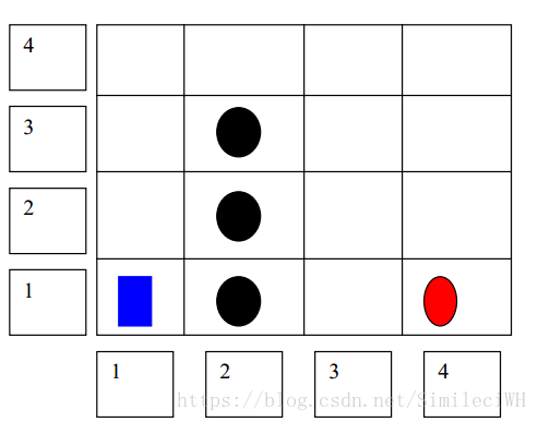
The robot (Blue Rectangle) has to traverse the terrain and reach the goal (the red Oval). A
brute force approach would be to start of with a square and identify all the squares that surround it.
Move to one of the successor square and repeat this process until the goal square is found.
However this method is computationally intensive and does not always guarantee the best

path to the target.

The key lies in identifying the appropriate successor square. Given some information
regarding the location of the target we can try to make an educated guess. For example if you know
your target lies to the east, explore squares to the east of your current location. If you know the

heading of the target you could always try to move to the square in that direction.

Can you come up with of a better way of determining which square needs to be selected?

A* uses the distance between the current location and the target and moves to the square
that has the smallest distance. It evaluates squares (henceforth called a “node”) by combining h(n),
the distance(cost ) to that node and g(n), the distance(cost) to get from that node to the goal node.
The total cost f (n) = g (n) +h (n) is calculated for each successor node and the node with the

smallest cost f (n) is selected as a successor.

1    Determining the Cost The distance between two nodes is simply determined by calculating the
straight distance between the two nodes. Though this might not the true distance (given the fact that
there are obstacles that need to be circumnavigated), it never overestimates the actual distance.
It can be shown that as long as cost is never overestimated, the algorithm is admissible i.e. it

generates the optimal path.

Let us consider the case for a simple 4X4 Matrix

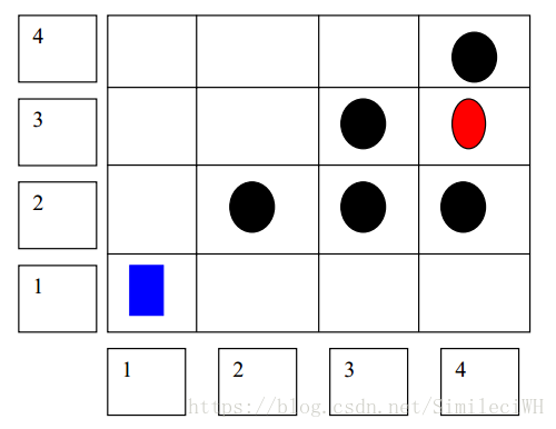
The start position is (1, 1). The successive node (only one in this case is (1, 2). There is no

ambiguity, until the Robot reaches node (2, 4). Here there are two nodes (3, 4) and (3, 3). The

successor node can be determined by evaluating the cost to the target from both the nodes.

f(n) for node (3, 3)

h(2,1) = 1 + 1 + sqrt(2) {Distance from N(1, 1) -> N(1,2) -> N(1,3)->N(2,1)}

f(n) = h(2, 1) + 1.414 (assuming each square is 1X1 units)

g(n) = sqrt( (4 – 3) ^2 + (1-3)^2) = 2.23

f(n)= 3.44+H(2,1)

f(n) for node (3,4)

h(n)= h(2,1) + 1

g(n)=sqrt( (4-3)^2 + (1-4)^2) = 4.16

        f(n) = 4.16 + h(2,1).

Now f(n) for (3,3) has been found to be the smallest of the two, hence the successor node is f(n).
The robot can now move to the node (3, 3) and continue expanding the successor nodes as above,

until the goal node is reached.

2    Dead End

What happens if the robot runs into a dead end? Consider the terrain

From what we have learnt so far Node (2, 1) will be chosen as the successor node instead of Node
(1, 2). The robot will continue to traverse the route until it ends up at the block at Node (4, 1).

We need to add a mechanism by which the robot:

a) Explores alternate routes once it lands up at a dead end.

b) Avoids traversing paths that it knows leads to a dead end.

This is done by maintaining two lists OPEN and CLOSED. The list OPEN stores all successive
paths that are yet to be explored while list CLOSED stores all paths that have been explored.
The list OPEN also stores the parent node of each node. This is used at the end to trace the path

from the Goal to the Start position, thus generating the optimal route.

Consider the figure below. The start node has 2 successors (2, 1) and (1, 2). From the initial
calculation (2, 1) is chosen and the robot travels along that node, however ones it reaches the dead
end, it discards the node (2, 1) and takes the second successor (1, 2) and explores that route.

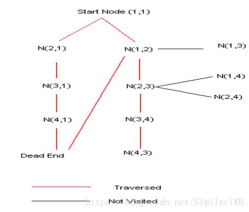
Once the goal node is reached the parent nodes are found and tracked back to the start node to get
the complete path.
In the above example N(4,3) -> N(3,4)->N(2,3)->N(1,2)->N(1,1) gives the optimal path.
From the above conditions the following algorithm can be obtained.

The A* Algorithm

1) Put the start node on the list OPEN and calculate the cost function f (n). {h (n) = 0; g(n) =

distance between the goal and the start position, f(n) = g(n).}

2) Remove from the List OPEN the node with the smallest cost function and put it on
CLOSED. This is the node n. (Incase two or more nodes have the cost function, arbitrarily

resolve ties. If one of the nodes is the goal node, then select the goal node)

3) If n is the goal node then terminate the algorithm and use the pointers to obtain the solution

path. Otherwise, continue

4) Determine all the successor nodes of n and compute the cost function for each successor not

on list CLOSED.

5) Associate with each successor not on list OPEN or CLOSED the cost calculated and put

these on the list OPEN, placing pointers to n (n is the parent node).

6) Associate with any successors already on OPEN the smaller of the cost values just

calculated and the previous cost value. ( min(new f(n), old f(n) ) )

7) Goto step 2.
3    Matlab Program
The Matlab Program consists of the following files
a) A_star1.m: This is the main file that contains the algorithm. This needs to be executed to
run the program.
b) distance.m: This is a function that calculates the distance between 2 nodes.
c) Expan_array.m: This function takes a node and returns the expanded list of successors, with
the calculated fn values. One of the criteria’s being none of the successors are on the
CLOSED list.
d) insert_open.m: This function populates the list OPEN with values that have been passed to
it. The arguments are xval,yval,parent_xval,parent_yval,hn,gn,fn .
e) min_fn.m: This function takes the list OPEN as one of its arguments and returns the node
with the smallest cost function.
f) Node_index.m: This function returns the index of the location of a node in the list OPEN.

以上所有内容非原创，皆是转载，仅供参考，可能存在一些问题。