word2vec实现cbow和skip-gram

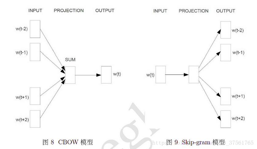
word2vec实现cbow和skip-gram

skip-gram

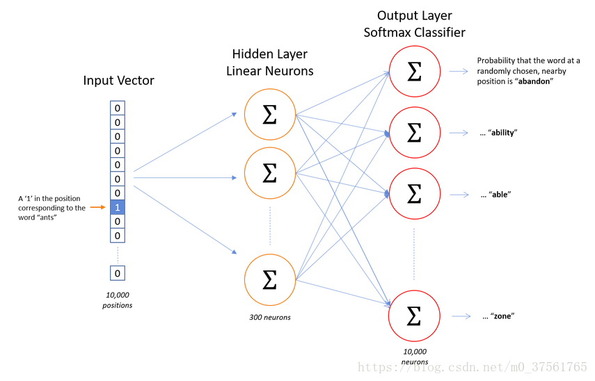
cbow

1.CBOW实现

"""
学习参考：
http://www.hankcs.com/ml/cbow-word2vec.html
https://blog.csdn.net/layumi1993/article/details/72866235
https://blog.csdn.net/linxuheng/article/details/70170888
"""
from __future__ import absolute_import
from __future__ import division
from __future__ import print_function

import collections
import math
import os
import random
import zipfile

os.environ["CUDA_VISIBLE_DEVICES"] = "9"

import numpy as np
from six.moves import urllib
from six.moves import xrange  # pylint: disable=redefined-builtin
import tensorflow as tf

# Step 1: Download the data.
url = 'http://mattmahoney.net/dc/'


def maybe_download(filename, expected_bytes):
    """Download a file if not present, and make sure it's the right size."""
    if not os.path.exists(filename):
        # 该方法返回一个包含两个元素的(filename, headers)元组，
        # filename 表示保存到本地的路径，header 表示服务器的响应头。
        filename, _ = urllib.request.urlretrieve(url + filename, filename)
    # stat 系统调用时用来返回相关文件的系统状态信息的。
    statinfo = os.stat(filename)
    # 文件的大小，以位为单位
    if statinfo.st_size == expected_bytes:
        print('Found and verified', filename)
    else:
        print(statinfo.st_size)
        raise Exception(
            'Failed to verify ' + filename + '. Can you get to it with a browser?')
    return filename


filename = maybe_download('text8.zip', 31344016)


# Read the data into a list of strings.
def read_data(filename):
    """Extract the first file enclosed in a zip file as a list of words"""
    with zipfile.ZipFile(filename) as f:
        #  英文字母读出来，分词，然后把分过后的词放在list中（str.split()可以做到）
        # [b'love', b'their', b'servitude', b'and',]
        data = tf.compat.as_str(f.read(f.namelist()[0])).split()
    return data


words = read_data(filename)
# size=17005207
print('Data size', len(words))

# Step 2: Build the dictionary and replace rare words with UNK token.
vocabulary_size = 50000


def build_dataset(words):
    count = [['UNK', -1]]
    # >>> c=Counter('dgfg')
    # >>> c
    # Counter({'g': 2, 'f': 1, 'd': 1})
    # >> > c.most_common(3)
    # [('r', 2), ('a', 1), ('g', 1)]
    count.extend(collections.Counter(words).most_common(vocabulary_size - 1))
    dictionary = dict()
    for word, _ in count:
        # 为词建立索引，词频越大，索引值越小。
        # {'g': 3, 'a': 2, 'UNK': 0, 'r': 1, 'p': 4}
        dictionary[word] = len(dictionary)
    data = list()
    unk_count = 0
    for word in words:
        if word in dictionary:
            index = dictionary[word]
        else:
            index = 0  # dictionary['UNK']
            unk_count += 1
        data.append(index)
    count[0][1] = unk_count
    reverse_dictionary = dict(zip(dictionary.values(), dictionary.keys()))
    # 建立50000个词的索引字典,这一步等同于为单词创建独热码(唯一的索引就可以写成one-hot的形式）
    #  data--》字典里词的索引值k形如[5239, 3083, 12, 6, 195, 2, 3134, 46, 59, 156]
    # count--》字典里词出现次数，词频[(‘UNK’,unk_count)，('r', 2), ('a', 1), ('g', 1)]
    # dictionary--》字典，包括词和词的索引k{'g': 3, 'a': 2, 'UNK': 0, 'r': 1, 'p': 4}
    # reverse_dictionary--》于字典相反，key是索引，value是词汇。{ 3：'g',  2：'a',  0：'UNK', 1：'r',4 :'p'}
    return data, count, dictionary, reverse_dictionary


data, count, dictionary, reverse_dictionary = build_dataset(words)
del words  # Hint to reduce memory.
print('Most common words (+UNK)', count[:5])
print('Sample data key:%sSample data:%s' % (data[:10], [reverse_dictionary[i] for i in data[:10]]))

data_index = 0

cbow_window = 1  # How many words to consider left and right.
# Step 3: Function to generate a training batch for the skip-gram model.
def generate_batch(batch_size,  cbow_window):
    global data_index
    # assert batch_size % num_skips == 0
    # assert num_skips <= 2 * bag_window
    span = 2 * cbow_window + 1  # 3 [ bag_window=1 ]
    batch = np.ndarray(shape=(batch_size,cbow_window*2), dtype=np.int32)
    # array([[0],
    #        [0],
    #        [353280],
    #        [1694499684],
    #        [40501248],
    #        [33587968],
    #        [1677722458],
    #        [55771140]], dtype=int32)
    labels = np.ndarray(shape=(batch_size, 1), dtype=np.int32)
    # deque双向列表
    buffer = collections.deque(maxlen=span)
    for _ in range(span):
        buffer.append(data[data_index])
        # 第1，2,3个词的索引值
        data_index = (data_index + 1) % len(data)
        '''
        每当有新的单词索引添加至缓冲区时，最左方的元素将从缓冲区中排出，
        以便为新的单词索引腾出空间。输入文本流中的缓冲器被存储在全局变量 data_index 中，
        每当缓冲器中有新的单词进入时， data_index 递增。
        如果到达文本流的末尾，索引更新的「％len（data）」组件会将计数重置为 0。

        '''
    for i in range(batch_size):
        target = cbow_window  # 1 target label at the center of the buffer
        targets_to_avoid = [cbow_window]
        # 从单词的 span
        # 范围中随机选择其他单词，确保上下文中不包含输入词且每个上下文单词都是唯一的。
        labels[i, 0] = buffer[cbow_window]
        # print("labels:",labels)
        for j in range(span-1):
                while target in targets_to_avoid:
                    #   0=<target<=2
                    target = random.randint(0, span - 1)
                targets_to_avoid.append(target)
                batch[i, j] = buffer[target]
                # print("batch:",batch)
        buffer.append(data[data_index])
        # print("data_index:",data_index)
        # print("data[data_index]",data[data_index])
        data_index = (data_index + 1) % len(data)
    return batch, labels


# batch(batch_size,2)是索引值，labels存的也是索引值[i,0]。
# [5243   12] -> 3084
batch, labels = generate_batch(batch_size=8,cbow_window=1)

for i in range(8):
    # anarchism originated as a term of abuse first used
    # [5243   12]['anarchism', 'as'] -> 3084 originated
    # [3084    6]['originated', 'a'] -> 12 as
    # [195  12]['term', 'as'] -> 6 a
    # [2 6]['of', 'a'] -> 195 term
    print( batch[i,:], [reverse_dictionary[batch[i,0]],
           reverse_dictionary[batch[i,1]]],

          '->', labels[i, 0], reverse_dictionary[labels[i, 0]])

# Step 4: Build and train a skip-gram model.

batch_size = 128  # 一次扫描多少块。
embedding_size = 128  # Dimension of the embedding vector.


# We pick a random validation set to sample nearest neighbors. Here we limit the
# validation samples to the words that have a low numeric ID, which by
# construction are also the most frequent.
'''
通过测量向量空间中最接近的向量来建立验证集，并使用英语知识以确保这些词确实是相似的。
这将在下一节中进行具体讨论。不过我们可以先暂时使用另一种方法，从词汇表最常用的词中随机提取验证单词，
上面的代码从 0 到 100 中随机选择了 16 个整数——这些整数与文本数据中最常用的 100 个单词的整数索引相对应。
https://blog.csdn.net/IAMoldpan/article/details/78707140
'''
valid_size = 16  # Random set of words to evaluate similarity on.
valid_window = 100  # Only pick dev samples in the head of the distribution.
# replace 默认为True允许采样有重复值，False不允许值重复，
# -->array([45, 85,  5, 59, 26, 75, 95, 84, 56,  7, 16, 78, 66,...]
valid_examples = np.random.choice(valid_window, valid_size, replace=False)
num_sampled = 64  # Number of negative examples to sample.

graph = tf.Graph()

with graph.as_default():
    # Input data.
    train_inputs = tf.placeholder(tf.int32, shape=[batch_size,cbow_window*2])
    train_labels = tf.placeholder(tf.int32, shape=[batch_size, 1])
    valid_dataset = tf.constant(valid_examples, dtype=tf.int32)

    # Ops and variables pinned to the CPU because of missing GPU implementation
    with tf.device('/cpu:0'):
        # Look up embeddings for inputs.
        # 参考解析look——up https://blog.csdn.net/u013041398/article/details/60955847
        embeddings = tf.Variable(
            tf.random_uniform([vocabulary_size, embedding_size], -1.0, 1.0))
        embed = tf.nn.embedding_lookup(embeddings, train_inputs)
        print('shape:',embed.get_shape())#shape: (128, 2, 128)
        # embeds = None
        # for i in range(2 * cbow_window):
        #     embedding_i = tf.nn.embedding_lookup(embeddings, train_inputs[:, i])
        #     print('embedding %d shape: %s' % (i, embedding_i.get_shape().as_list()))
        #     emb_x, emb_y = embedding_i.get_shape().as_list()
        #     if embeds is None:
        #         embeds = tf.reshape(embedding_i, [emb_x, emb_y, 1])
        #     else:
        #         embeds = tf.concat([embeds, tf.reshape(embedding_i, [emb_x, emb_y, 1])],2)
        #
        # assert embeds.get_shape().as_list()[2] == 2 * cbow_window
        # print("Concat embedding size: %s" % embeds.get_shape().as_list())
        # avg_embed = tf.reduce_mean(embeds, 2, keep_dims=False)
        # print("Avg embedding size: %s" % avg_embed.get_shape().as_list())

        # Construct the variables for the NCE loss
        nce_weights = tf.Variable(
            tf.truncated_normal([vocabulary_size, embedding_size],
                                stddev=1.0 / math.sqrt(embedding_size)))
        nce_biases = tf.Variable(tf.zeros([vocabulary_size]))
        # '''
        # 原始的写法，用softmax判断,时间略长。
        # '''
        # （batch_size=128,vocabulary_size=50000）
        # hidden_out = tf.matmul(embed, tf.transpose(nce_weights)) + nce_biases
        # one_hot_labels=tf.one_hot(tf.reshape(train_labels,[batch_size]),depth=vocabulary_size)
        # loss=tf.reduce_mean(tf.nn.softmax_cross_entropy_with_logits(labels=one_hot_labels, logits=hidden_out,
        #                                   name=None))
    # Compute the average NCE loss for the batch.
    # tf.nce_loss automatically draws a new sample of the negative labels each
    # time we evaluate the loss.
    loss = tf.reduce_mean(
        tf.nn.nce_loss(nce_weights, nce_biases, tf.cast(train_labels, tf.float32), tf.reduce_mean(embed,1),
                       num_sampled, vocabulary_size))

    # Construct the SGD optimizer using a learning rate of 1.0.
    optimizer = tf.train.GradientDescentOptimizer(1.0).minimize(loss)

    # Compute the cosine similarity between minibatch examples and all embeddings.
    norm = tf.sqrt(tf.reduce_sum(tf.square(embeddings), 1, keep_dims=True))
    normalized_embeddings = embeddings / norm
    valid_embeddings = tf.nn.embedding_lookup(
        normalized_embeddings, valid_dataset)
    # 该操作将返回一个（validation_size, vocabulary_size）大小的张量，
    # 该张量的每一行指代一个验证词，列则指验证词和词汇表中其他词的相似度。
    # (16,50000)
    similarity = tf.matmul(
        valid_embeddings, normalized_embeddings, transpose_b=True)

    # Add variable initializer.
    init = tf.initialize_all_variables()

# Step 5: Begin training.
num_steps = 100001

with tf.Session(graph=graph) as session:
    # We must initialize all variables before we use them.
    init.run()
    print("Initialized")

    average_loss = 0
    for step in xrange(num_steps):
        batch_inputs, batch_labels = generate_batch(
            batch_size, cbow_window)
        feed_dict = {train_inputs: batch_inputs, train_labels: batch_labels}

        # We perform one update step by evaluating the optimizer op (including it
        # in the list of returned values for session.run()
        _, loss_val = session.run([optimizer, loss], feed_dict=feed_dict)
        average_loss += loss_val

        if step % 2000 == 0:
            if step > 0:
                average_loss /= 2000
            # The average loss is an estimate of the loss over the last 2000 batches.
            print("Average loss at step ", step, ": ", average_loss)
            average_loss = 0

        # Note that this is expensive (~20% slowdown if computed every 500 steps)
        if step % 10000 == 0:
            sim = similarity.eval()
            for i in xrange(valid_size):
                valid_word = reverse_dictionary[valid_examples[i]]
                top_k = 8  # number of nearest neighbors
                # argsort()
                # 函数是将x中的元素从小到大排列，提取其对应的index(索引)，
                # 从1开始到第9个是因为分数最高的一定是自己，把自己排除。
                nearest = (-sim[i, :]).argsort()[1:top_k + 1]
                log_str = "Nearest to %s:" % valid_word
                for k in xrange(top_k):
                    close_word = reverse_dictionary[nearest[k]]
                    log_str = "%s %s," % (log_str, close_word)
                print(log_str)
    final_embeddings = normalized_embeddings.eval()


# Step 6: Visualize the embeddings.

def plot_with_labels(low_dim_embs, labels, filename='tsne.png'):
    assert low_dim_embs.shape[0] >= len(labels), "More labels than embeddings"
    plt.figure(figsize=(18, 18))  # in inches
    for i, label in enumerate(labels):
        x, y = low_dim_embs[i, :]
        plt.scatter(x, y)
        plt.annotate(label,
                     xy=(x, y),
                     xytext=(5, 2),
                     textcoords='offset points',
                     ha='right',
                     va='bottom')

    plt.savefig(filename)


try:
    from sklearn.manifold import TSNE
    import matplotlib.pyplot as plt

    tsne = TSNE(perplexity=30, n_components=2, init='pca', n_iter=5000)
    plot_only = 500
    low_dim_embs = tsne.fit_transform(final_embeddings[:plot_only, :])
    labels = [reverse_dictionary[i] for i in xrange(plot_only)]
    plot_with_labels(low_dim_embs, labels)

except ImportError:
    print("Please install sklearn, matplotlib, and scipy to visualize embeddings.")

Average loss at step  92000 :  4.13854655159
Average loss at step  94000 :  4.20275877428
Average loss at step  96000 :  4.14698807251
Average loss at step  98000 :  3.88556081307
Average loss at step  100000 :  3.90406033587
Nearest to years: internet, days, stages, whitcomb, alban, analyzing, positivism, alley,
Nearest to have: had, has, were, are, require, be, never, ifrcs,
Nearest to called: gel, martens, given, fin, tsar, predetermined, comnenus, believers,
Nearest to use: mesoplodon, measure, electrical, most, study, welt, gysin, thereafter,
Nearest to state: producer, soil, accomplishments, callithrix, duchy, government, mississippi, story,
Nearest to or: and, structuring, mythos, than, insular, scratch, hint, prix,
Nearest to it: he, she, this, there, usages, they, herbert, what,
Nearest to some: many, several, all, these, lucid, blended, functionally, those,
Nearest to also: still, often, always, generally, steep, never, adopted, originally,
Nearest to after: before, when, during, ddrmax, kerr, aurangzeb, from, climbing,
Nearest to would: will, could, can, may, should, must, might, cannot,
Nearest to be: been, is, was, become, are, have, were, matter,
Nearest to other: different, arthritis, various, pertwee, plasma, guderian, herbaceous, lagrange,
Nearest to than: or, facing, shrugged, much, nyu, annealing, elmo, inducing,
Nearest to this: which, it, our, albums, joaquin, bet, any, grass,
Nearest to these: those, many, such, some, various, all, enchanted, they,
Please install sklearn, matplotlib, and scipy to visualize embeddings.

2.skip-gram实现
同tensorflow下的word2vec_basic,进行了注释，加了softmax+entropy 熵的情况，对英文文本中的句子进行实现，

"""
学习参考：
https://blog.csdn.net/sweetcandy2/article/details/73351031
https://www.jianshu.com/p/f682066f0586
https://www.jiqizhixin.com/articles/2017-11-20-3
"""
from __future__ import absolute_import
from __future__ import division
from __future__ import print_function

import collections
import math
import os
import random
import zipfile
os.environ["CUDA_VISIBLE_DEVICES"] = "9"

import numpy as np
from six.moves import urllib
from six.moves import xrange  # pylint: disable=redefined-builtin
import tensorflow as tf

# Step 1: Download the data.
url = 'http://mattmahoney.net/dc/'

def maybe_download(filename, expected_bytes):
  """Download a file if not present, and make sure it's the right size."""
  if not os.path.exists(filename):
    # 该方法返回一个包含两个元素的(filename, headers)元组，
    # filename 表示保存到本地的路径，header 表示服务器的响应头。
    filename, _ = urllib.request.urlretrieve(url + filename, filename)
  #stat 系统调用时用来返回相关文件的系统状态信息的。
  statinfo = os.stat(filename)
  # 文件的大小，以位为单位
  if statinfo.st_size == expected_bytes:
    print('Found and verified', filename)
  else:
    print(statinfo.st_size)
    raise Exception(
        'Failed to verify ' + filename + '. Can you get to it with a browser?')
  return filename

filename = maybe_download('text8.zip', 31344016)


# Read the data into a list of strings.
def read_data(filename):
  """Extract the first file enclosed in a zip file as a list of words"""
  with zipfile.ZipFile(filename) as f:
    #  英文字母读出来，分词，然后把分过后的词放在list中（str.split()可以做到）
    # [b'love', b'their', b'servitude', b'and',]
    data = tf.compat.as_str(f.read(f.namelist()[0])).split()
  return data

words = read_data(filename)
# size=17005207
print('Data size', len(words))

# Step 2: Build the dictionary and replace rare words with UNK token.
vocabulary_size = 50000

def build_dataset(words):
  count = [['UNK', -1]]
  # >>> c=Counter('dgfg')
  # >>> c
  # Counter({'g': 2, 'f': 1, 'd': 1})
  # >> > c.most_common(3)
  # [('r', 2), ('a', 1), ('g', 1)]
  count.extend(collections.Counter(words).most_common(vocabulary_size - 1))
  dictionary = dict()
  for word, _ in count:
    # 为词建立索引，词频越大，索引值越小。
    # {'g': 3, 'a': 2, 'UNK': 0, 'r': 1, 'p': 4}
    dictionary[word] = len(dictionary)
  data = list()
  unk_count = 0
  for word in words:
    if word in dictionary:
      index = dictionary[word]
    else:
      index = 0  # dictionary['UNK']
      unk_count += 1
    data.append(index)
  count[0][1] = unk_count
  reverse_dictionary = dict(zip(dictionary.values(), dictionary.keys()))
  # 建立50000个词的索引字典,这一步等同于为单词创建独热码(唯一的索引就可以写成one-hot的形式）
  #  data--》字典里词的索引值k形如[5239, 3083, 12, 6, 195, 2, 3134, 46, 59, 156]
  # count--》字典里词出现次数，词频[(‘UNK’,unk_count)，('r', 2), ('a', 1), ('g', 1)]
  # dictionary--》字典，包括词和词的索引k{'g': 3, 'a': 2, 'UNK': 0, 'r': 1, 'p': 4}
  # reverse_dictionary--》于字典相反，key是索引，value是词汇。{ 3：'g',  2：'a',  0：'UNK', 1：'r',4 :'p'}
  return data, count, dictionary, reverse_dictionary

data, count, dictionary, reverse_dictionary = build_dataset(words)
del words  # Hint to reduce memory.
print('Most common words (+UNK)', count[:5])
print('Sample data key:%sSample data:%s'% (data[:10], [reverse_dictionary[i] for i in data[:10]]))

data_index = 0


# Step 3: Function to generate a training batch for the skip-gram model.
def generate_batch(batch_size, num_skips, skip_window):
  global data_index
  assert batch_size % num_skips == 0
  assert num_skips <= 2 * skip_window
  # batch=array([0, 0, 91136, 1694499428, 40501248,
  #        33587968, 1677722458, 5439491], dtype=int32)
  batch = np.ndarray(shape=(batch_size), dtype=np.int32)
  # array([[0],
  #        [0],
  #        [353280],
  #        [1694499684],
  #        [40501248],
  #        [33587968],
  #        [1677722458],
  #        [55771140]], dtype=int32)
  labels = np.ndarray(shape=(batch_size, 1), dtype=np.int32)
  span = 2 * skip_window + 1 #3 [ skip_window target skip_window ]
  # deque双向列表
  buffer = collections.deque(maxlen=span)
  for _ in range(span):
    buffer.append(data[data_index])
    # 第1，2,3个词的索引值
    data_index = (data_index + 1) % len(data)
    '''
    每当有新的单词索引添加至缓冲区时，最左方的元素将从缓冲区中排出，
    以便为新的单词索引腾出空间。输入文本流中的缓冲器被存储在全局变量 data_index 中，
    每当缓冲器中有新的单词进入时， data_index 递增。
    如果到达文本流的末尾，索引更新的「％len（data）」组件会将计数重置为 0。

    '''
  for i in range(batch_size // num_skips):
    target = skip_window  # 1 target label at the center of the buffer
    targets_to_avoid = [ skip_window ]
    # 从单词的 span
    # 范围中随机选择其他单词，确保上下文中不包含输入词且每个上下文单词都是唯一的。
    for j in range(num_skips):
      while target in targets_to_avoid:
        #   0=<target<=2
        target = random.randint(0, span - 1)
      targets_to_avoid.append(target)
      batch[i * num_skips + j] = buffer[skip_window]
      labels[i * num_skips + j, 0] = buffer[target]
    buffer.append(data[data_index])
    data_index = (data_index + 1) % len(data)
  return batch, labels
# batch[i]是索引值，labels存的也是索引值[i,0]。
batch, labels = generate_batch(batch_size=8, num_skips=2, skip_window=1)
for i in range(8):
  # anarchism originated as a term of abuse first used
  # 3083 originated -> 5239 anarchism
  # 12 as -> 6 a
  # 12 as -> 3083 originated
  print(batch[i], reverse_dictionary[batch[i]],
      '->', labels[i, 0], reverse_dictionary[labels[i, 0]])

# Step 4: Build and train a skip-gram model.

batch_size = 128 #一次扫描多少块。
embedding_size = 128  # Dimension of the embedding vector.
skip_window = 1       # How many words to consider left and right.
num_skips = 2         # How many times to reuse an input to generate a label.

# We pick a random validation set to sample nearest neighbors. Here we limit the
# validation samples to the words that have a low numeric ID, which by
# construction are also the most frequent.
'''
通过测量向量空间中最接近的向量来建立验证集，并使用英语知识以确保这些词确实是相似的。
这将在下一节中进行具体讨论。不过我们可以先暂时使用另一种方法，从词汇表最常用的词中随机提取验证单词，
上面的代码从 0 到 100 中随机选择了 16 个整数——这些整数与文本数据中最常用的 100 个单词的整数索引相对应。
https://blog.csdn.net/IAMoldpan/article/details/78707140
'''
valid_size = 16     # Random set of words to evaluate similarity on.
valid_window = 100  # Only pick dev samples in the head of the distribution.
#replace 默认为True允许采样有重复值，False不允许值重复，
# -->array([45, 85,  5, 59, 26, 75, 95, 84, 56,  7, 16, 78, 66,...]
valid_examples = np.random.choice(valid_window, valid_size, replace=False)
num_sampled = 64    # Number of negative examples to sample.

graph = tf.Graph()

with graph.as_default():

  # Input data.
  train_inputs = tf.placeholder(tf.int32, shape=[batch_size])
  train_labels = tf.placeholder(tf.int32, shape=[batch_size, 1])
  valid_dataset = tf.constant(valid_examples, dtype=tf.int32)

  # Ops and variables pinned to the CPU because of missing GPU implementation
  with tf.device('/cpu:0'):
    # Look up embeddings for inputs.
    # 参考解析look——up https://blog.csdn.net/u013041398/article/details/60955847
    embeddings = tf.Variable(
        tf.random_uniform([vocabulary_size, embedding_size], -1.0, 1.0))
    embed = tf.nn.embedding_lookup(embeddings, train_inputs)

    # Construct the variables for the NCE loss
    nce_weights = tf.Variable(
        tf.truncated_normal([vocabulary_size, embedding_size],
                            stddev=1.0 / math.sqrt(embedding_size)))
    nce_biases = tf.Variable(tf.zeros([vocabulary_size]))
    # '''
    # 原始的写法，用softmax判断,时间略长。
    # '''
    # # （batch_size=128,vocabulary_size=50000）
    # hidden_out = tf.matmul(embed, tf.transpose(nce_weights)) + nce_biases
    # one_hot_labels=tf.one_hot(tf.reshape(train_labels,[batch_size]),depth=vocabulary_size)
    # loss=tf.reduce_mean(tf.nn.softmax_cross_entropy_with_logits(labels=one_hot_labels, logits=hidden_out,
    #                                   name=None))
  # Compute the average NCE loss for the batch.
  # tf.nce_loss automatically draws a new sample of the negative labels each
  # time we evaluate the loss.
  loss = tf.reduce_mean(
      tf.nn.nce_loss(nce_weights, nce_biases, tf.cast( train_labels,tf.float32),embed,
                     num_sampled, vocabulary_size))

  # Construct the SGD optimizer using a learning rate of 1.0.
  optimizer = tf.train.GradientDescentOptimizer(1.0).minimize(loss)

  # Compute the cosine similarity between minibatch examples and all embeddings.
  norm = tf.sqrt(tf.reduce_sum(tf.square(embeddings), 1, keep_dims=True))
  normalized_embeddings = embeddings / norm
  valid_embeddings = tf.nn.embedding_lookup(
      normalized_embeddings, valid_dataset)
  # 该操作将返回一个（validation_size, vocabulary_size）大小的张量，
  # 该张量的每一行指代一个验证词，列则指验证词和词汇表中其他词的相似度。
  # (16,50000)
  similarity = tf.matmul(
      valid_embeddings, normalized_embeddings, transpose_b=True)

  # Add variable initializer.
  init = tf.initialize_all_variables()

# Step 5: Begin training.
num_steps = 100001

with tf.Session(graph=graph) as session:
  # We must initialize all variables before we use them.
  init.run()
  print("Initialized")

  average_loss = 0
  for step in xrange(num_steps):
    batch_inputs, batch_labels = generate_batch(
        batch_size, num_skips, skip_window)
    feed_dict = {train_inputs : batch_inputs, train_labels : batch_labels}

    # We perform one update step by evaluating the optimizer op (including it
    # in the list of returned values for session.run()
    _, loss_val = session.run([optimizer, loss], feed_dict=feed_dict)
    average_loss += loss_val

    if step % 2000 == 0:
      if step > 0:
        average_loss /= 2000
      # The average loss is an estimate of the loss over the last 2000 batches.
      print("Average loss at step ", step, ": ", average_loss)
      average_loss = 0

    # Note that this is expensive (~20% slowdown if computed every 500 steps)
    if step % 10000 == 0:
      sim = similarity.eval()
      for i in xrange(valid_size):
        valid_word = reverse_dictionary[valid_examples[i]]
        top_k = 8 # number of nearest neighbors
        # argsort()
        # 函数是将x中的元素从小到大排列，提取其对应的index(索引)，
        # 从1开始到第9个是因为分数最高的一定是自己，把自己排除。
        nearest = (-sim[i, :]).argsort()[1:top_k+1]
        log_str = "Nearest to %s:" % valid_word
        for k in xrange(top_k):
          close_word = reverse_dictionary[nearest[k]]
          log_str = "%s %s," % (log_str, close_word)
        print(log_str)
  final_embeddings = normalized_embeddings.eval()

# Step 6: Visualize the embeddings.

def plot_with_labels(low_dim_embs, labels, filename='tsne.png'):
  assert low_dim_embs.shape[0] >= len(labels), "More labels than embeddings"
  plt.figure(figsize=(18, 18))  #in inches
  for i, label in enumerate(labels):
    x, y = low_dim_embs[i,:]
    plt.scatter(x, y)
    plt.annotate(label,
                 xy=(x, y),
                 xytext=(5, 2),
                 textcoords='offset points',
                 ha='right',
                 va='bottom')

  plt.savefig(filename)

try:
  from sklearn.manifold import TSNE
  import matplotlib.pyplot as plt

  tsne = TSNE(perplexity=30, n_components=2, init='pca', n_iter=5000)
  plot_only = 500
  low_dim_embs = tsne.fit_transform(final_embeddings[:plot_only,:])
  labels = [reverse_dictionary[i] for i in xrange(plot_only)]
  plot_with_labels(low_dim_embs, labels)

except ImportError:
  print("Please install sklearn, matplotlib, and scipy to visualize embeddings.")

Average loss at step  92000 :  4.70792403448
Average loss at step  94000 :  4.61834581614
Average loss at step  96000 :  4.73397651279
Average loss at step  98000 :  4.61884291029
Average loss at step  100000 :  4.68271846807
Nearest to however: but, and, although, that, which, abitibi, when, though,
Nearest to first: last, agouti, second, stench, next, formidable, cerebral, abet,
Nearest to was: is, has, had, were, became, been, by, being,
Nearest to world: mitral, commuters, swims, erectus, dmd, peculiarities, largest, ssbn,
Nearest to three: four, five, two, six, seven, eight, callithrix, zero,
Nearest to in: during, at, on, abitibi, within, and, throughout, from,
Nearest to during: in, after, at, from, into, against, under, when,
Nearest to d: b, thaler, dasyprocta, section, immolation, alum, connecticut, groves,
Nearest to six: seven, eight, four, five, nine, three, two, zero,
Nearest to UNK: callithrix, dasyprocta, tamarin, upanija, reginae, iit, cebus, four,
Nearest to its: their, his, the, her, sheridan, microcebus, galvani, hooke,
Nearest to only: agouti, quine, callithrix, casuistry, microcebus, hypotension, prism, tamarin,
Nearest to united: redfern, successor, clodius, provocation, touring, upanija, treachery, of,
Nearest to for: dasyprocta, agouti, prism, with, during, tamarin, while, towards,
Nearest to been: be, was, were, by, become, pontificia, had, always,
Nearest to th: eight, seven, six, four, nine, frud, two, allotropes,
Please install sklearn, matplotlib, and scipy to visualize embeddings.

同tensorflow下的word2vec_basic,进行了注释，加了softmax+entropy 熵的情况，对中文文本中的句子进行实现，那么就有分词的问题，选用合工大LTP。

Average loss at step  92000 :  4.19266751575
Average loss at step  94000 :  4.10320964313
Average loss at step  96000 :  4.11487320387
Average loss at step  98000 :  4.06696178246
Average loss at step  100000 :  4.10072786987
nearest: [ 5049 25731   169  2964   508 28401    38   347]
Nearest to 有着: 收取, 饺子, 因为, 不乏, 掠过, 一步之遥, 有, 拥有,
nearest: [  652   639   321   435 17367 18282   324    79]
Nearest to 道: 丝, 问道, 一道道, 怔, 反之, 落日, 枚, 声,
nearest: [  178   865   364 11195 16746  1153 22879 20820]
Nearest to 有些: 极为, 异常, 颇为, 对得起, 安安稳稳, 显, 魂殿待, 假体,
nearest: [  123  2706   629  1082  2614    47  7785 45052]
Nearest to 点: 摇, ☆, 松, 一番, ♀, 笑, ┅, ......................................,
nearest: [   71  5245  4610  3547  9404  6424  8918 11426]
Nearest to 上: 之上, 干瘦, 气浪, 绝, 黄莲精, 漠城, 天上, ︴,
nearest: [ 2706 11715 11426 23616  7785  6967  5496 10970]
Nearest to UNK: ☆, ♂, ︴, 第两百九十八, ┅, 功, 黑夜, 攻击性,
nearest: [  485   389  1009   912   160 11797  5185   159]
Nearest to 目光: 视线, 眼睛, 美眸, 眼神, 声音, ①, 怒喝道, 脸色,
nearest: [   1  116 2706    3   77 7785    9 2614]
Nearest to ,: ，, ’, ☆, 。, …, ┅, ”, ♀,
nearest: [ 142  334  105  148   76 2614  102 5124]
Nearest to 这种: 这个, 那种, 这些, 这般, 一些, ♀, 什么, 逛,
nearest: [  175   150 11715   663 10929 18793    57  2706]
Nearest to 出: 出来, 进, ♂, 幕, 囦体, 燃, 去, ☆,
nearest: [  31   18  260   59   94  166  266 2706]
Nearest to 你: 我, 他, 你们, 他们, 她, 我们, 它, ☆,
nearest: [  28  154  257 2706    9  126  140  211]
Nearest to “: ！, 听, 闻, ☆, ”, 见到, 对于, 随着,
nearest: [  403   472   673 11426   366   991   435   610]
Nearest to 笑: 苦笑, 微笑, 叹, ︴, 冷笑, 挥手, 怔, 咬,
nearest: [  132   438  8028   142 12533 36092 15307  8744]
Nearest to 一个: 个, 那个, 不动声色, 这个, 印射, 魂断涧, 大斗篷, 阻挡,
nearest: [  86 5732  143 1505 6795 7554   63 9404]
Nearest to 最后: 然后, 左, 如今, 长枪, 皱褶, 裔民, 旋即, 黄莲精,
nearest: [  118   162 16797 14389   256   318 14924  2947]
Nearest to 般: 一般, 犹如, 煞殿, 迈进, 如, 如同, 诀窍, 身材,