NLP | Word2Vec之基于Hierarchical Softmax的 skip-gram 和 CBOW 模型

版权声明：本文为博主原创文章，未经博主允许不得转载，欢迎大家讨论交流。 https://blog.csdn.net/qq_40006058/article/details/86423862

主要介绍Word2Vec中的Skip-Gram模型和CBOW模型。总结来说，skip-gram是用中心词预测周围词，预测的时候是一对word pair，等于对每一个中心词都有K个词作为output，对于一个词的预测有K次，所以能够更有效的从context中学习信息，但是总共预测K*V词。CBOW模型中input是context（周围词），而output是中心词。因此，skip gram的训练时间更长，但是对于一些出现频率不高的词，在CBOW中的学习效果就不日skip-gram。

1 Skip-gram

假如我们有一个句子“The dog barked at the mailman”。

1. 首先，我们选句子中间的一个词作为我们的输入词，例如我们选取“dog”作为input word；
2. 然后，有了input word以后，我们再定义一个叫做skip_window的参数，它代表着我们从当前input word的一侧（左边或右边）选取词的数量。如果skip_window=2，那么我们最终获得窗口中的词（包括input word在内）就是**[‘The’, ‘dog’，‘barked’, ‘at’]**。skip_window=2代表着选取左input word左侧2个词和右侧2个词进入我们的窗口，所以整个窗口大小span=2x2=4。另一个参数叫num_skips，它代表着我们从整个窗口中选取多少个不同的词作为我们的output word，当skip_window=2，num_skips=2时，我们将会得到两组(input word, output word)形式的训练数据，即(‘dog’, ‘barked’)，(‘dog’, ‘the’)。
3. 最后，神经网络基于这些训练数据将会输出一个概率分布，这个概率代表着我们的词典中的每个词是output word的可能性。这句话有点绕，我们来看个栗子。第二步中我们在设置skip_window和num_skips=2的情况下获得了两组训练数据。假如我们先拿一组数据 (‘dog’, ‘barked’)来训练神经网络，那么模型通过学习这个训练样本，会告诉我们词汇表中每个单词是“barked”的概率大小。

选定句子“The quick brown fox jumps over lazy dog”，设定我们的窗口大小为2（window_size=2），也就是说我们仅选输入词前后各两个词和输入词进行组合。下图中，蓝色代表input word，方框内代表位于窗口内的单词。

模型细节

我们如何来表示这些单词呢？
首先，我们都知道神经网络只能接受数值输入，我们不可能把一个单词字符串作为输入，因此我们得想个办法来表示这些单词。最常用的办法就是基于训练文档来构建我们自己的词汇表（vocabulary）再对单词进行one-hot编码。

假设从我们的训练文档中抽取出10000个唯一不重复的单词组成词汇表。我们对这10000个单词进行one-hot编码，得到的每个单词都是一个10000维的向量，向量每个维度的值只有0或者1，假如单词ants在词汇表中的出现位置为第3个，那么ants的向量就是一个第三维度取值为1，其他维都为0的10000维的向量（ants=[0,0, 1, 0, …, 0]）。还是上面的例子，“The dog barked at the mailman”，那么我们基于这个句子，可以构建一个大小为5的词汇表（忽略大小写和标点符号）：(“the”, “dog”, “barked”, “at”, “mailman”)，我们对这个词汇表的单词进行编号0-4。那么”dog“就可以被表示为一个5维向量[0,1, 0, 0, 0]。

模型的输入如果为一个10000维的向量，那么输出也是一个10000维度（词汇表的大小）的向量，它包含了10000个概率，每一个概率代表着当前词是输入样本中output word的概率大小。

隐层

隐层没有使用任何激活函数，但是输出层使用了sotfmax。我们基于成对的单词来对神经网络进行训练，训练样本是 ( input word,output word ) 这样的单词对，input word和output word都是one-hot编码的向量。最终模型的输出是一个概率分布。

如果我们现在想用300个特征来表示一个单词（即每个词可以被表示为300维的向量）。那么隐层的权重矩阵应该为10000行，300列（隐层有300个结点）。Google在最新发布的基于Google news数据集训练的模型中使用的就是300个特征的词向量。词向量的维度是一个可以调节的超参数（在Python的gensim包中封装的Word2Vec接口默认的词向量大小为100， window_size为5）。

看下面的图片，左右两张图分别从不同角度代表了输入层-隐层的权重矩阵。左图中每一列代表一个10000维的词向量和隐层单个神经元连接的权重向量。从右边的图来看，每一行实际上代表了每个单词的词向量。

所以我们最终的目标就是学习这个隐层的权重矩阵。我们现在回来接着通过模型的定义来训练我们的这个模型。上面我们提到，input word和output word都会被我们进行one-hot编码。仔细想一下，我们的输入被one-hot编码以后大多数维度上都是0（实际上仅有一个位置为1），所以这个向量相当稀疏，那么会造成什么结果呢。如果我们将一个1 x 10000的向量和10000 x 300的矩阵相乘，它会消耗相当大的计算资源，为了高效计算，它仅仅会选择矩阵中对应的向量中维度值为1的索引行（这句话很绕），看图就明白。

我们来看一下上图中的矩阵运算，左边分别是1 x 5和5 x 3的矩阵，结果应该是1 x 3的矩阵，按照矩阵乘法的规则，结果的第一行第一列元素为0 x 17 + 0 x 23 + 0 x 4 + 1 x 10 + 0 x 11 = 10，同理可得其余两个元素为12，19。如果10000个维度的矩阵采用这样的计算方式是十分低效的。

为了有效地进行计算，这种稀疏状态下不会进行矩阵乘法计算，可以看到矩阵的计算的结果实际上是矩阵对应的向量中值为1的索引，上面的例子中，左边向量中取值为1的对应维度为3（下标从0开始），那么计算结果就是矩阵的第3行（下标从0开始）—— [10, 12, 19]，这样模型中的隐层权重矩阵便成了一个”查找表“（lookup table），进行矩阵计算时，直接去查输入向量中取值为1的维度下对应的那些权重值。隐层的输出就是每个输入单词的“嵌入词向量”。

输出层
经过神经网络隐层的计算，ants这个词会从一个1 x 10000的向量变成1 x 300的向量，再被输入到输出层。输出层是一个softmax回归分类器，它的每个结点将会输出一个0-1之间的值（概率），这些所有输出层神经元结点的概率之和为1。下面是一个例子，训练样本为 (input word: “ants”， output word: “car”) 的计算示意图。

Tensorflow 实现Skip-gram（电影评分数据集）

导入所需的库

# 导入库
from tensorflow.python.framework import ops
ops.reset_default_graph()
import tensorflow as tf
sess = tf.Session()
import matplotlib.pyplot as plt
import numpy as np
import random
import os # OS模块可以处理文件和目录这些我们日常手动需要做的操作。
import string # 可以调用与字符串操作相关的函数。
import requests # requests是python的一个HTTP客户端库
import collections
"""
collections提供了一下数据类型，很厉害
1.namedtuple(): 生成可以使用名字来访问元素内容的tuple子类
2.deque: 双端队列，可以快速的从另外一侧追加和推出对象
3.Counter: 计数器，主要用来计数
4.OrderedDict: 有序字典
5.defaultdict: 带有默认值的字典
"""
import io #  'StringIO',BytesIO',...
import gzip
import tarfile # 压缩、解压
import urllib.request
"""
Urllib是python内置的HTTP请求库包括以下模块
urllib.request 请求模块
urllib.error 异常处理模块
urllib.parse url解析模块
urllib.robotparser robots.txt解析模块
"""
from nltk.corpus import stopwords

声明一些模型参数

batch_size = 50 # 一次查找50对词嵌套。
embedding_size = 200 # 每个单词嵌套大小为长度200的向量。
vocabulary_size = 10000 # 仅考虑频次为10000的单词
generations = 50000 # 迭代训练50000次
print_loss_every = 500 # 迭代500次打印一次损失函数
num_sampled = int(batch_size/2) # Number of negative examples to sample.
window_size = 3 # 查找目标单词两边各两个上下文单词
stops = stopwords.words('english')
print_valid_every = 2000 # 每迭代2000次训练打印最近邻域单词
valid_words = ['cliche', 'love', 'hate', 'silly', 'sad']

数据加载。首先检验是否已经下载了数据，如果下载了就直接加载就行，没有下载的话就去下载

def load_movie_data():
    save_folder_name = 'temp'
    pos_file = os.path.join(save_folder_name, 'rt-polaritydata', 'rt-polarity.pos')
    neg_file = os.path.join(save_folder_name, 'rt-polaritydata', 'rt-polarity.neg')
    if not os.path.exists(os.path.join(save_folder_name, 'rt-polaritydata')):
        movie_data_url = 'http://www.cs.cornell.edu/people/pabo/movie-review-data/rt-polaritydata.tar.gz'
        req = requests.get(movie_data_url, stream=True)
        with open('temp_movie_review_temp.tar.gz', 'wb') as f:
            for chunk in req.iter_content(chunk_size=1024):
                if chunk:
                    f.write(chunk)
                    f.flush()
        # Extract tar.gz file into temp folder
        tar = tarfile.open('temp_movie_review_temp.tar.gz', "r:gz")
        tar.extractall(path='temp')
        tar.close()
    pos_data = []
    with open(pos_file, 'r', encoding='latin-1') as f:
        for line in f:
            pos_data.append(line.encode('ascii', errors='ignore').decode())
    f.close()
    pos_data = [x.rstrip() for x in pos_data]
    neg_data = []
    with open(neg_file, 'r', encoding='latin-1') as f:
        for line in f:
            neg_data.append(line.encode('ascii', errors='ignore').decode())
    f.close()
    neg_data = [x.rstrip() for x in neg_data] # Python rstrip() 删除 string 字符串末尾的指定字符（默认为空格
    texts = pos_data + neg_data
    target = [1] * len(pos_data) + [0] * len(neg_data)
    return texts, target
texts, target = load_movie_data()

结果：
[‘the rock is destined to be the 21st century’s new " conan " and that he’s going to make a splash even greater than arnold schwarzenegger , jean-claud van damme or steven segal .’, ‘the gorgeously elaborate continuation of " the lord of the rings " trilogy is so huge that a column of words cannot adequately describe co-writer/director peter jackson’s expanded vision of j . r . r . tolkien’s middle-earth .’, ‘effective but too-tepid biopic’, ‘if you sometimes like to go to the movies to have fun , wasabi is a good place to start .’, “emerges as something rare , an issue movie that’s so honest and keenly observed that it doesn’t feel like one .”]
[1, 1, 1, 1, 1]

创建归一化文本函数。大小写、标点、数字、空格、停用词

def normalize_text(texts, stopwords):
    texts = [x.lower() for x in texts]
    texts = [''.join(x for x in text if x not in string.punctuation) for text in texts]
    print(texts[0:2])
    print("---------------------------------------------------------------------------------------")
    texts = [''.join(x for x in text if x not in '0123456789') for text in texts]
    print(texts[0:2])
    print("---------------------------------------------------------------------------------------")
    texts = [' '.join([word for word in text.split() if word not in stops]) for text in texts]
    print(texts[0:2])
    print("---------------------------------------------------------------------------------------")
    texts = [' '.join(text.split()) for text in texts]
    return texts
texts = normalize_text(texts, stops)
print(texts[0:5])

输出结果：
['the rock is destined to be the 21st centurys new conan and that hes going to make a splash even greater than arnold schwarzenegger jeanclaud van damme or steven segal ', 'the gorgeously elaborate continuation of the lord of the rings trilogy is so huge that a column of words cannot adequately describe cowriterdirector peter jacksons expanded vision of j r r tolkiens middleearth ']

['the rock is destined to be the st centurys new conan and that hes going to make a splash even greater than arnold schwarzenegger jeanclaud van damme or steven segal ', 'the gorgeously elaborate continuation of the lord of the rings trilogy is so huge that a column of words cannot adequately describe cowriterdirector peter jacksons expanded vision of j r r tolkiens middleearth ']

[‘rock destined st centurys new conan hes going make splash even greater arnold schwarzenegger jeanclaud van damme steven segal’, ‘gorgeously elaborate continuation lord rings trilogy huge column words cannot adequately describe cowriterdirector peter jacksons expanded vision j r r tolkiens middleearth’]

[‘rock destined st centurys new conan hes going make splash even greater arnold schwarzenegger jeanclaud van damme steven segal’, ‘gorgeously elaborate continuation lord rings trilogy huge column words cannot adequately describe cowriterdirector peter jacksons expanded vision j r r tolkiens middleearth’, ‘effective tootepid biopic’, ‘sometimes like go movies fun wasabi good place start’, ‘emerges something rare issue movie thats honest keenly observed doesnt feel like one’]

为了确保影评的有效性，强制影评长度大于等于三个单词。然后构建词汇表，从而实现{word:频次}的映射

target = [target[ix] for ix,x in enumerate(texts) if len(x.split()) > 2]
texts = [x for x in texts if len(x.split()) > 2]

# 构建词汇表，创建函数来建立一个单词字典（单词和单词数对），词频不够的单词标记为RARE
def build_dictionary(sentences, vocabulary_size):
    # Turn sentences (list of strings) into lists of words
    split_sentences = [s.split() for s in sentences]
    print(split_sentences[0:5])
    print("=============================================================")
    words = [x for sublist in split_sentences for x in sublist]
    print(words[0:5])
    print("=============================================================")
    # Initialize list of [word, word_count] for each word, starting with unknown
    count = [['RARE', -1]]
    # Now add most frequent words, limited to the N-most frequent (N=vocabulary size)
    count.extend(collections.Counter(words).most_common(vocabulary_size - 1))
    # Now create the dictionary
    word_dict = {}
    # For each word, that we want in the dictionary, add it, then make it
    # the value of the prior dictionary length
    for word, word_count in count:
        word_dict[word] = len(word_dict)
    return word_dict
word_dict = build_dictionary(texts, vocabulary_size)
for k, v in word_dict.items():
    print(k + ":" + str(v))

输出结果：
[[‘rock’, ‘destined’, ‘st’, ‘centurys’, ‘new’, ‘conan’, ‘hes’, ‘going’, ‘make’, ‘splash’, ‘even’, ‘greater’, ‘arnold’, ‘schwarzenegger’, ‘jeanclaud’, ‘van’, ‘damme’, ‘steven’, ‘segal’], [‘gorgeously’, ‘elaborate’, ‘continuation’, ‘lord’, ‘rings’, ‘trilogy’, ‘huge’, ‘column’, ‘words’, ‘cannot’, ‘adequately’, ‘describe’, ‘cowriterdirector’, ‘peter’, ‘jacksons’, ‘expanded’, ‘vision’, ‘j’, ‘r’, ‘r’, ‘tolkiens’, ‘middleearth’], [‘effective’, ‘tootepid’, ‘biopic’], [‘sometimes’, ‘like’, ‘go’, ‘movies’, ‘fun’, ‘wasabi’, ‘good’, ‘place’, ‘start’], [‘emerges’, ‘something’, ‘rare’, ‘issue’, ‘movie’, ‘thats’, ‘honest’, ‘keenly’, ‘observed’, ‘doesnt’, ‘feel’, ‘like’, ‘one’]]

[‘rock’, ‘destined’, ‘st’, ‘centurys’, ‘new’]

thats:39
idiocy:4039
tenacious:5294
stand:685
authenticity:3966
worry:3967
familial:3092
。。。此处省略10000字。。。

将一系列的句子转化成单词索引列表，并将单词索引列表传入嵌套寻找函数

def text_to_numbers(sentences, word_dict):
    data = []
    for sentence in sentences:
        sentence_data = []
        for word in sentence:
            if word in word_dict:
                word_ix = word_dict[word]
            else:
                word_ix = 0
            sentence_data.append(word_ix)
        data.append(sentence_data)
    return data

# 创建单词字典、转换句子列表为单词索引列表
word_dictionary = build_dictionary(texts, vocabulary_size)
word_dictionary_rev = dict(zip(word_dictionary.values(), word_dictionary.keys())) # 键值互换
text_data = text_to_numbers(texts, word_dictionary)
print(text_data[0:5])
# 从预处理的单词词典中查找用于验证的单词的索引
valid_examples = [word_dictionary[x] for x in valid_words]

print(valid_examples)
print(word_dictionary["rock"])
print(word_dictionary_rev[546])

[[2708, 0, 1872, 1044, 0, 0, 753, 0, 0, 0, 2408, 753, 0, 0, 0, 0, 0, 1872, 753, 2408, 0, 1775, 2708, 0, 0, 0, 2408, 753, 2754, 0, 1872, 0, 2408, 0, 2408, 0, 2044, 753, 0, 0, 2637, 0, 0, 2408, 2637, 0, 0, 0, 1044, 753, 0, 0, 4294, 4227, 0, 0, 2044, 0, 753, 8725, 753, 2408, 0, 2637, 2708, 753, 0, 0, 753, 2708, 0, 0, 2708, 2408, 0, 4227, 0, 0, 0, 1872, 2044, 2754, 0, 2708, 0, 753, 2408, 753, 2637, 2637, 753, 2708, 0, 1150, 753, 0, 2408, 1872, 4227, 0, 1775, 0, 0, 8725, 0, 2408, 0, 0, 0, 0, 0, 753, 0, 0, 0, 753, 8725, 753, 2408, 0, 0, 753, 2637, 0, 4227], [2637, 0, 2708, 2637, 753, 0, 1775, 0, 4227, 0, 0, 753, 4227, 0, 1363, 0, 2708, 0, 0, 753, 0, 1872, 0, 2408, 0, 0, 2408, 1775, 0, 0, 0, 0, 2408, 0, 4227, 0, 2708, 0, 0, 2708, 0, 2408, 2637, 0, 0, 0, 2708, 0, 4227, 0, 2637, 0, 0, 2044, 1775, 2637, 753, 0, 1872, 0, 4227, 1775, 0, 2408, 0, 2754, 0, 2708, 0, 0, 0, 1872, 0, 2408, 2408, 0, 0, 0, 0, 0, 753, 2864, 1775, 0, 0, 753, 4227, 0, 0, 0, 753, 0, 1872, 2708, 0, 1363, 753, 0, 1872, 0, 2754, 2708, 0, 0, 753, 2708, 0, 0, 2708, 753, 1872, 0, 0, 2708, 0, 4294, 753, 0, 753, 2708, 0, 1150, 0, 1872, 1044, 0, 0, 2408, 0, 0, 753, 979, 4294, 0, 2408, 0, 753, 0, 0, 8725, 0, 0, 0, 0, 2408, 0, 1150, 0, 2708, 0, 2708, 0, 0, 0, 4227, 1044, 0, 753, 2408, 0, 0, 0, 0, 0, 0, 4227, 753, 753, 0, 2708, 0, 2044], [753, 9010, 9010, 753, 1872, 0, 0, 8725, 753, 0, 0, 0, 0, 0, 753, 4294, 0, 0, 0, 1363, 0, 0, 4294, 0, 1872], [0, 0, 0, 753, 0, 0, 0, 753, 0, 0, 4227, 0, 1044, 753, 0, 2637, 0, 0, 0, 0, 8725, 0, 753, 0, 0, 9010, 1775, 2408, 0, 2754, 0, 0, 0, 1363, 0, 0, 2637, 0, 0, 0, 0, 4294, 4227, 0, 1872, 753, 0, 0, 0, 0, 2708, 0], [753, 0, 753, 2708, 2637, 753, 0, 0, 0, 0, 0, 753, 0, 2044, 0, 2408, 2637, 0, 2708, 0, 2708, 753, 0, 0, 0, 0, 1775, 753, 0, 0, 0, 8725, 0, 753, 0, 0, 2044, 0, 0, 0, 0, 2044, 0, 2408, 753, 0, 0, 0, 1044, 753, 753, 2408, 4227, 0, 0, 0, 1363, 0, 753, 2708, 8725, 753, 0, 0, 0, 0, 753, 0, 2408, 0, 0, 9010, 753, 753, 4227, 0, 4227, 0, 1044, 753, 0, 0, 2408, 753]]

[1423, 28, 952, 200, 360]

546

rock

创建skip-gram模型的批量函数。希望在单词对上训练模型，第一个单词作为输入（目标单词），另一个单词作为输出。比如“the cat in the hat”，目标单词为in， 上下文窗口大小设置为2，那么训练单词对为（in, the）, (in, cat), (in, the), (in, hat)。
需要注意：窗口大小为2的话包含四个单词，前面讲的四个单词中包含目标单词，而代码里包含除目标单词外的另四个单词（也就是五个单词）。其实也不影响理解。

# 创建函数返回skip-gram模型的批量数据
def generate_batch_data(sentences, batch_size, window_size, method='skip-gram'):
    batch_data = []
    label_data = []
    while len(batch_data) < batch_size:
        rand_sentence = np.random.choice(sentences) # 随机选择一个开始
        window_sequences = [rand_sentence[max((ix-window_size),0):(ix+window_size+1)] for ix,x in enumerate(rand_sentence)]
        label_indices = [ix if ix<window_size else window_size for ix,x in enumerate(window_sequences)] # 寻找中心点单词
        # 为每个窗口取出中心感兴趣的单词，并为每个窗口创建一个元组
        if method == 'skip-gram': # 从目标单词预测上下文
            batch_and_labels = [(x[y],x[:y]+x[(y+1):]) for x,y in zip(window_sequences,label_indices)] 
            tuple_data = [(x,y_) for x,y in batch_and_labels for y_ in y] # (target word, surrounding word)
        elif method == 'cbow': # 利用上下文预测目标单词
            batch_and_labels = [(x[:y]+x[(y+1):],x[y]) for x,y in zip(window_sequences,label_indices)] # (target word, surrounding word)
            tuple_data = [(x_, y) for x, y in batch_and_labels for x_ in x]# (target word, surrounding word)
        else:
            raise ValueError('Method {} not implemented yet.'.format(method))
        batch,labels = [list(x) for x in zip(*tuple_data)] # 提取batch和label
        batch_data.extend(batch[:batch_size])
        label_data.extend(labels[:batch_size])
    batch_data = batch_data[:batch_size] # 在结尾处修剪批次和标签
    label_data = label_data[:batch_size]
    batch_data = np.array(batch_data)
    label_data = np.transpose(np.array([label_data]))
    return batch_data,label_data
batch_data, label_data = generate_batch_data(text_data, batch_size, window_size, method='skip-gram')

for i in range(4):
    print(str(batch_data[i+8]) + ' ' + str(label_data[i+8]))

输出结果：
0 [2408]
0 [0]
0 [4294]
0 [753]

初始化嵌套矩阵，声明占位符和嵌套从查找函数

# 初始化嵌套矩阵
embeddings = tf.Variable(tf.random_uniform([vocabulary_size, embedding_size]))

# 创建占位符
x_inputs = tf.placeholder(tf.int32, shape=[batch_size])
y_target = tf.placeholder(tf.int32, shape=[batch_size, 1])
valid_dataset = tf.constant(valid_examples, dtype=tf.int32)

# 嵌套查找函数
embed = tf.nn.embedding_lookup(embeddings, x_inputs)

softmax是实现多分类常用的损失函数，但是本例目标是10000个不同的分类，稀疏性非常高，导致算法模型拟合或收敛的问题。为了解决这个问题使用噪声对比损失函数NCE。NCE损失函数将问题转化成一个二值预测，预测单词分类和随机噪声。

# NCE损失函数
nce_weights = tf.Variable(tf.truncated_normal([vocabulary_size, embedding_size],
                                              stddev=1.0 / np.sqrt(embedding_size)))
nce_biases = tf.Variable(tf.zeros([vocabulary_size]))

# Get loss from prediction
loss = tf.reduce_mean(tf.nn.nce_loss(weights=nce_weights,
                                     biases=nce_biases,
                                     labels=y_target,
                                     inputs=embed,
                                     num_sampled=num_sampled,
                                     num_classes=vocabulary_size))

通过计算单词集与所有词向量之间的余弦相似度寻找验证单词周围的单词

norm = tf.sqrt(tf.reduce_sum(tf.square(embeddings), 1, keepdims=True))
normalized_embeddings = embeddings / norm
valid_embeddings = tf.nn.embedding_lookup(normalized_embeddings, valid_dataset)
similarity = tf.matmul(valid_embeddings, normalized_embeddings, transpose_b=True)

声明优化器函数，初始化模型变量

# Create optimizer
optimizer = tf.train.GradientDescentOptimizer(learning_rate=1.0).minimize(loss)

# Add variable initializer.
init = tf.global_variables_initializer()
sess.run(init)

迭代训练单词嵌套

loss_vec = []
loss_x_vec = []
for i in range(generations):
    batch_inputs, batch_labels = generate_batch_data(text_data, batch_size, window_size)
    feed_dict = {x_inputs: batch_inputs, y_target: batch_labels}

    # Run the train step
    sess.run(optimizer, feed_dict=feed_dict)

    # Return the loss
    if (i + 1) % print_loss_every == 0:
        loss_val = sess.run(loss, feed_dict=feed_dict)
        loss_vec.append(loss_val)
        loss_x_vec.append(i+1)
        print('Loss at step {} : {}'.format(i+1, loss_val))
      
    # Validation: Print some random words and top 5 related words
    if (i+1) % print_valid_every == 0:
        sim = sess.run(similarity, feed_dict=feed_dict)
        for j in range(len(valid_words)):
            valid_word = valid_words[j]
            # top_k = number of nearest neighbors
            top_k = 5
            nearest = (-sim[j, :]).argsort()[1:top_k+1]
            log_str = "Nearest to {}:".format(valid_word)
            for k in range(top_k):
                close_word = word_dictionary_rev[nearest[k]]
                log_str = '{} {},'.format(log_str, close_word)
            print(log_str)

输出结果：
。。。。。。此处略去10000字 。。。。。。。。。。
Loss at step 48500 : 1.0923460721969604
Loss at step 49000 : 0.956238865852356
Loss at step 49500 : 0.19344420731067657
Loss at step 50000 : 1.9008288383483887
Nearest to cliche: enticing, mcgrath, media, hitandmiss, guiltypleasure,
Nearest to love: witty, rant, punchdrunk, brisk, scene,
Nearest to hate: commerce, cannot, proven, constant, triste,
Nearest to silly: dramatization, wellshot, fabulous, tuned, death,
Nearest to sad: chouchou, tomcats, enduring, kicking, patric,

CBOW—连续词袋模型

CBOW的神经网络模型与skip-gram的神经网络模型也是互为镜像的。

现在的Corpus是这一个简单的只有四个单词的document：{I drink coffee everyday}，我们选coffee作为中心词，window size设为2。也就是说，我们要根据单词"I","drink"和"everyday"来预测一个单词，并且我们希望这个单词是coffee。

输入层：上下文单词的onehot14维3个词

输出层：1*4维的向量（概率表示）

ram模型的输入输出是相反的。这里输入层是由one-hot编码的输入上下文{ ${x_1,…,x_C}$}组成，其中窗口大小为 $C$，词汇表大小为 $V$。隐藏层是 $N$维的向量。最后输出层是也被one-hot编码的输出单词 $y$。被one-hot编码的输入向量通过一个 $V×N$维的权重矩阵 $W$连接到隐藏层；隐藏层通过一个 $N×V$的权重矩阵 $W′$连接到输出层。

接下来，我们假设我们知道输入与输出权重矩阵的大小。

1. 第一步就是去计算隐藏层 $h$的输出。如下：
   $h = \frac{1}{C}W\cdot (\sum_{i=1}^C x_i)\tag{$1$}$
   该输出就是输入向量的加权平均。这里的隐藏层与skip-gram的隐藏层明显不同。

2. 第二部就是计算在输出层每个结点的输入。如下:
   $u_{j}=v^{'T}_{wj}\cdot h\tag{$2$}$
   其中 $v^{'T}_{wj}$是输出矩阵 $W^′$的第 $j$列。

3. 最后我们计算输出层的输出，输出 $y_j$如下：
   $y_{c,j} =p(w_{y,j}|w_1,...,w_c) = \frac{exp(u_{j})}{\sum^V_{j^{'}=1}exp(u^{'}j)}\tag{$3$}$

通过BP（反向传播）算法及随机梯度下降来学习权重

在学习权重矩阵 $W$与 $W′$过程中，我们可以给这些权重赋一个随机值来初始化。然后按序训练样本，逐个观察输出与真实值之间的误差，并计算这些误差的梯度。并在梯度方向纠正权重矩阵。这种方法被称为随机梯度下降。但这个衍生出来的方法叫做反向传播误差算法。

import tensorflow as tf
import matplotlib.pyplot as plt
import numpy as np
import random
import os
import pickle
import string
import requests
import collections
import io
import tarfile
import urllib.request
from nltk.corpus import stopwords
from tensorflow.python.framework import ops
ops.reset_default_graph()

tf.set_random_seed(42)
np.random.seed(42)

data_folder_name = 'temp'
if not os.path.exists(data_folder_name):
    os.makedirs(data_folder_name)

sess = tf.Session()

batch_size = 500
embedding_size = 200
vocabulary_size = 2000
generations = 50000
model_learning_rate = 0.25
num_sampled = int(batch_size/2)    # Number of negative examples to sample.
window_size = 3       # How many words to consider left and right.
save_embeddings_every = 5000
print_valid_every = 5000
print_loss_every = 100
stops = stopwords.words('english')
valid_words = ['love', 'hate', 'happy', 'sad', 'man', 'woman']

# Normalize text
def normalize_text(texts, stops):
    texts = [x.lower() for x in texts]
    texts = [''.join(c for c in x if c not in string.punctuation) for x in texts]
    texts = [''.join(c for c in x if c not in '0123456789') for x in texts]
    texts = [' '.join([word for word in x.split() if word not in (stops)]) for x in texts]
    texts = [' '.join(x.split()) for x in texts]
    return(texts)

# Build dictionary of words
def build_dictionary(sentences, vocabulary_size):
    split_sentences = [s.split() for s in sentences] # split_sentences 格式[['dw','dqw',...,'dqw'],[......]]
    words = [x for sublist in split_sentences for x in sublist]
    count = [['RARE', -1]]
    count.extend(collections.Counter(words).most_common(vocabulary_size-1))
    word_dict = {}
    for word, word_count in count:
        word_dict[word] = len(word_dict)  
    return(word_dict)
    
# Turn text data into lists of integers from dictionary
def text_to_numbers(sentences, word_dict):
    data = []
    for sentence in sentences:
        sentence_data = []
        for word in sentence.split(' '):
            if word in word_dict:
                word_ix = word_dict[word]
            else:
                word_ix = 0
            sentence_data.append(word_ix)
        data.append(sentence_data)
    return(data)
    
# Generate data randomly (N words behind, target, N words ahead)
def generate_batch_data(sentences, batch_size, window_size, method='skip_gram'):
    batch_data = []
    label_data = []
    while len(batch_data) < batch_size:
        rand_sentence_ix = int(np.random.choice(len(sentences), size=1))
        rand_sentence = sentences[rand_sentence_ix]
        window_sequences = [rand_sentence[max((ix-window_size),0):(ix+window_size+1)] for ix, x in enumerate(rand_sentence)]
        # Denote which element of each window is the center word of interest
        label_indices = [ix if ix<window_size else window_size for ix,x in enumerate(window_sequences)]
        # Pull out center word of interest for each window and create a tuple for each window
        batch, labels = [], []
        if method=='skip_gram':
            batch_and_labels = [(x[y], x[:y] + x[(y+1):]) for x,y in zip(window_sequences, label_indices)]
            # Make it in to a big list of tuples (target word, surrounding word)
            tuple_data = [(x, y_) for x,y in batch_and_labels for y_ in y]
            if len(tuple_data) > 0:
                batch, labels = [list(x) for x in zip(*tuple_data)]
        elif method=='cbow':
            batch_and_labels = [(x[:y] + x[(y+1):], x[y]) for x,y in zip(window_sequences, label_indices)]
            # Only keep windows with consistent 2*window_size
            batch_and_labels = [(x,y) for x,y in batch_and_labels if len(x)==2*window_size]
            if len(batch_and_labels) > 0:
                batch, labels = [list(x) for x in zip(*batch_and_labels)]
        elif method=='doc2vec':
            # For doc2vec we keep LHS window only to predict target word
            batch_and_labels = [(rand_sentence[i:i+window_size], rand_sentence[i+window_size]) for i in range(0, len(rand_sentence)-window_size)]
            batch, labels = [list(x) for x in zip(*batch_and_labels)]
            # Add document index to batch!! Remember that we must extract the last index in batch for the doc-index
            batch = [x + [rand_sentence_ix] for x in batch]
        else:
            raise ValueError('Method {} not implemented yet.'.format(method))
        # extract batch and labels
        batch_data.extend(batch[:batch_size])
        label_data.extend(labels[:batch_size])
    # Trim batch and label at the end
    batch_data = batch_data[:batch_size]
    label_data = label_data[:batch_size]
    # Convert to numpy array
    batch_data = np.array(batch_data)
    label_data = np.transpose(np.array([label_data]))
    return batch_data, label_data

# Load the movie review data
# Check if data was downloaded, otherwise download it and save for future use
def load_movie_data():
    save_folder_name = 'temp'
    pos_file = os.path.join(save_folder_name, 'rt-polaritydata', 'rt-polarity.pos')
    neg_file = os.path.join(save_folder_name, 'rt-polaritydata', 'rt-polarity.neg')

    # Check if files are already downloaded
    if not os.path.exists(os.path.join(save_folder_name, 'rt-polaritydata')):
        movie_data_url = 'http://www.cs.cornell.edu/people/pabo/movie-review-data/rt-polaritydata.tar.gz'

        # Save tar.gz file
        req = requests.get(movie_data_url, stream=True)
        with open('temp_movie_review_temp.tar.gz', 'wb') as f:
            for chunk in req.iter_content(chunk_size=1024):
                if chunk:
                    f.write(chunk)
                    f.flush()
        # Extract tar.gz file into temp folder
        tar = tarfile.open('temp_movie_review_temp.tar.gz', "r:gz")
        tar.extractall(path='temp')
        tar.close()
    pos_data = []
    with open(pos_file, 'r', encoding='latin-1') as f:
        for line in f:
            pos_data.append(line.encode('ascii',errors='ignore').decode())
    f.close()
    pos_data = [x.rstrip() for x in pos_data]
    neg_data = []
    with open(neg_file, 'r', encoding='latin-1') as f:
        for line in f:
            neg_data.append(line.encode('ascii',errors='ignore').decode())
    f.close()
    neg_data = [x.rstrip() for x in neg_data]
    texts = pos_data + neg_data
    target = [1]*len(pos_data) + [0]*len(neg_data)
    return(texts, target)

data_folder_name = 'temp'
if not os.path.exists(data_folder_name):
    os.makedirs(data_folder_name)
    
texts, target = load_movie_data()
texts = normalize_text(texts, stops)
target = [target[ix] for ix,x in enumerate(texts) if len(x.split()) > 2]
texts = [x for x in texts if len(x.split()) > 2]

# 创建单词字典，以便查找单词
word_dictionary = build_dictionary(texts, vocabulary_size)
word_dictionary_rev = dict(zip(word_dictionary.values(), word_dictionary.keys()))
text_data = text_to_numbers(texts, word_dictionary)
valid_examples = [word_dictionary[word] for word in valid_words]

# 初始化待拟合的单词嵌套并声明算法模型的数据占位符
embeddings = tf.Variable(tf.random_uniform([vocabulary_size, embedding_size], -1., 1.))
x_inputs = tf.placeholder(shape=[batch_size, 2*window_size], dtype=tf.int32)
y_target = tf.placeholder(shape=[batch_size, 1], dtype=tf.int32)
valid_dataset = tf.constant(valid_examples, dtype=tf.int32)

# 处理单词嵌套
embed = tf.zeros([batch_size, embedding_size])
for element in range(2*window_size):
    embed += tf.nn.embedding_lookup(embeddings, x_inputs[:,element])
   
# NCE损失函数
nce_weights = tf.Variable(tf.truncated_normal([vocabulary_size,embedding_size], stddev=1.0/np.sqrt(embedding_size)))
nce_bias = tf.Variable(tf.zeros(vocabulary_size))
loss = tf.reduce_mean(tf.nn.nce_loss(weights=nce_weights,
                                     biases=nce_bias,
                                     labels=y_target,
                                     inputs=embed,
                                     num_sampled=num_sampled,
                                     num_classes=vocabulary_size))

# 利用余弦相似度度量最接近的单词
norm = tf.sqrt(tf.reduce_sum(tf.square(embeddings), 1, keep_dims=True))
normalized_embeddings = embeddings / norm
valid_embeddings = tf.nn.embedding_lookup(normalized_embeddings, valid_dataset)
similarity = tf.matmul(valid_embeddings,normalized_embeddings,transpose_b=True )

# 保存词向量
saver = tf.train.Saver({"embeddings":embeddings})

# 声明优化器函数，初始化变量
optmizer = tf.train.GradientDescentOptimizer(learning_rate=model_learning_rate).minimize(loss)
init = tf.global_variables_initializer()
sess.run(init)

# 遍历迭代、打印损失函数、保存单词嵌套
loss_vec = []
loss_x_vec = []
text_data = [x for x in text_data if len(x)>=(2*window_size+1)]
for i in range(generations):
    batch_inputs, batch_labels = generate_batch_data(text_data,batch_size,window_size,method="cbow")
    feed_dict = {x_inputs:batch_inputs, y_target:batch_labels}
    sess.run(optmizer, feed_dict=feed_dict)
    if (i+1) % print_loss_every == 0:
        loss_val = sess.run(loss, feed_dict=feed_dict)
        loss_vec.append(loss_val)
        loss_x_vec.append(i+1)
        print('loss at step {}:{}'.format(i+1,loss_val))
    if (i+1) % print_valid_every == 0:
        sim = sess.run(similarity, feed_dict=feed_dict)
        for j in range(len(valid_words)):
            valid_word = word_dictionary_rev[valid_examples[j]]
            top_k = 5
            nearest = (-sim[j,:]).argsort()[1:top_k+1]
            log_str = "Nearest to {}".format(valid_word)
            for k in range(top_k):
                close_word = word_dictionary_rev[nearest[k]]
                print_str = '{} {}'.format(log_str, close_word)
            print(print_str)
    if (i+1) % save_embeddings_every == 0:
        with open(os.path.join(data_folder_name, 'movie_vocab.pkl'), 'wb') as f:
            pickle.dump(word_dictionary, f)
        model_checkpoint_path = os.path.join(os.getcwd(), data_folder_name, 'cbow_movie_embeddings.ckpt')
        save_path = saver.save(sess, model_checkpoint_path)
        print('Model saved in file: {}'.format(save_path))

输出结果：
。。。。。。。。此处省略一万字。。。。。。.。。。
loss at step 49200:2.3909201622009277
loss at step 49300:2.5774049758911133
loss at step 49400:2.058192491531372
loss at step 49500:2.1763217449188232
loss at step 49600:2.239227056503296
loss at step 49700:2.235402822494507
loss at step 49800:2.0298542976379395
loss at step 49900:2.2141225337982178
loss at step 50000:2.3587381839752197
Nearest to love side
Nearest to hate talent
Nearest to happy taste
Nearest to sad energy
Nearest to man irritating
Nearest to woman chemistry
Model saved in file: D:\anaconda\envs\tensorflow\Scripts\Tensorflow机器学习实战指南\temp\cbow_movie_embeddings.ckpt

理论基础

参考资料

1. Skip-Gram模型理解
2. An Intuitive Understanding of Word Embeddings: From Count Vectors
   to Word2Vec这一篇非常赞，介绍了embeddings的两种基本形式以及每种形式下的代表方法。
3. 轻松理解CBOW
4. word2vec中CBOW和Skip-Gram训练模型的原理
   
5. CBOW与Skip-Gram模型基础
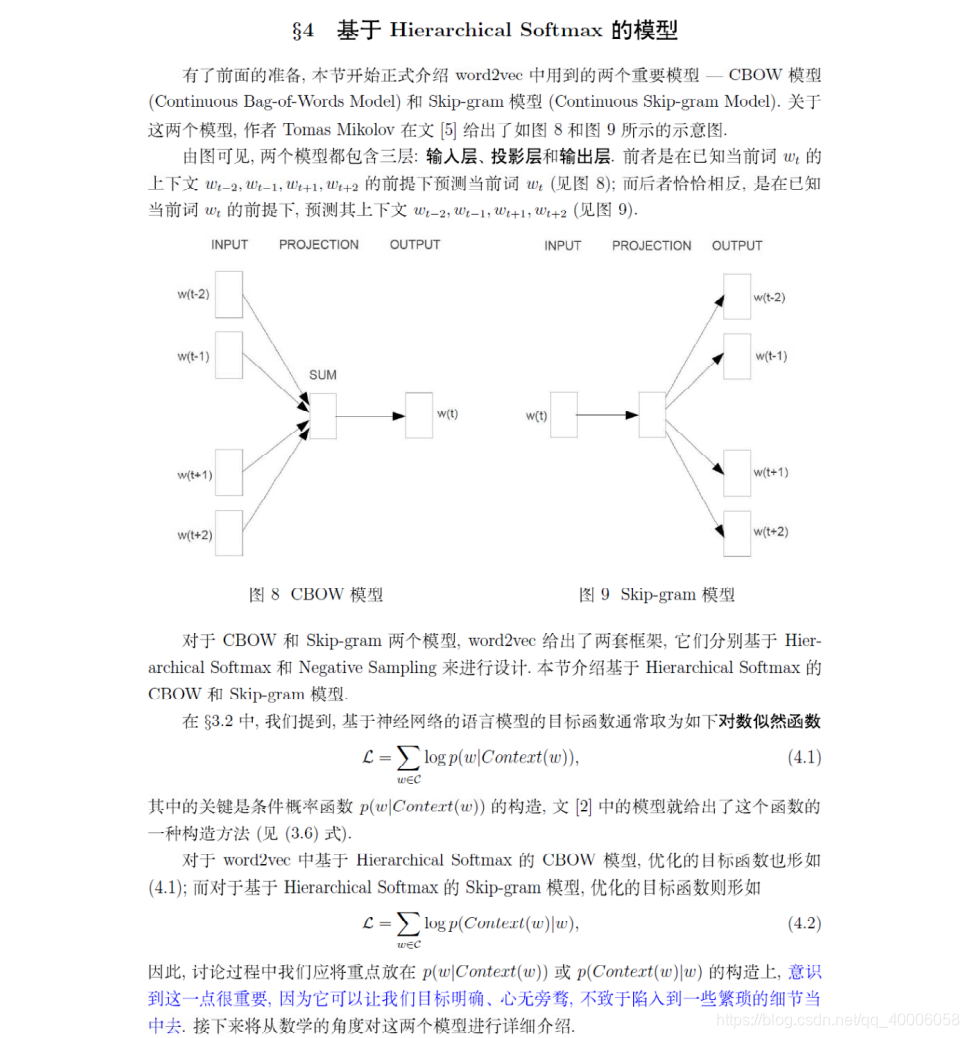
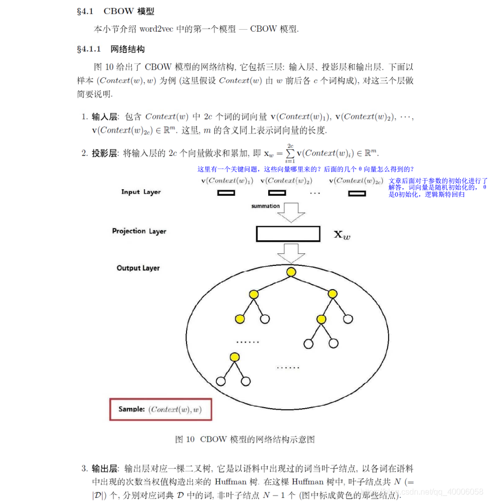
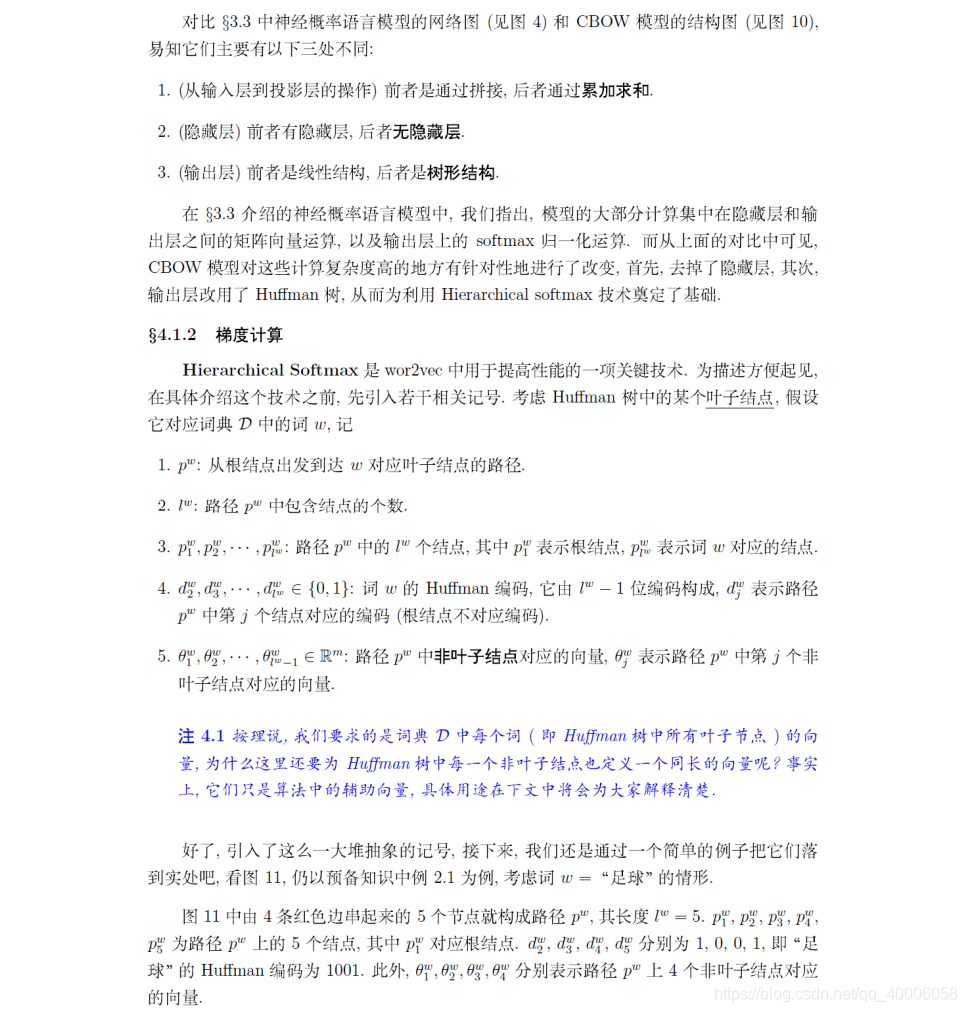
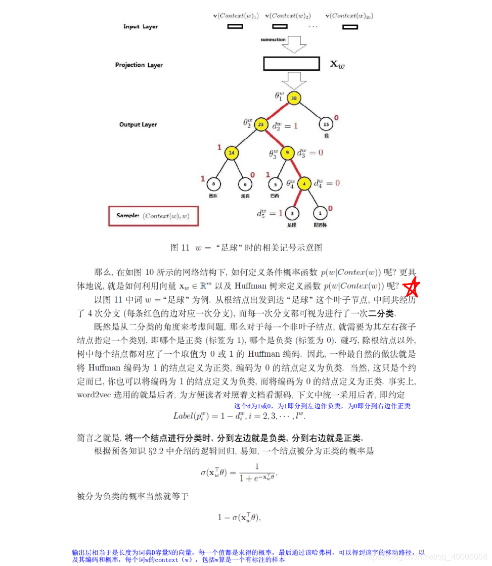
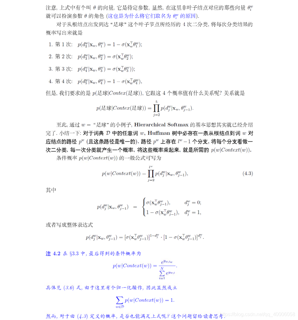
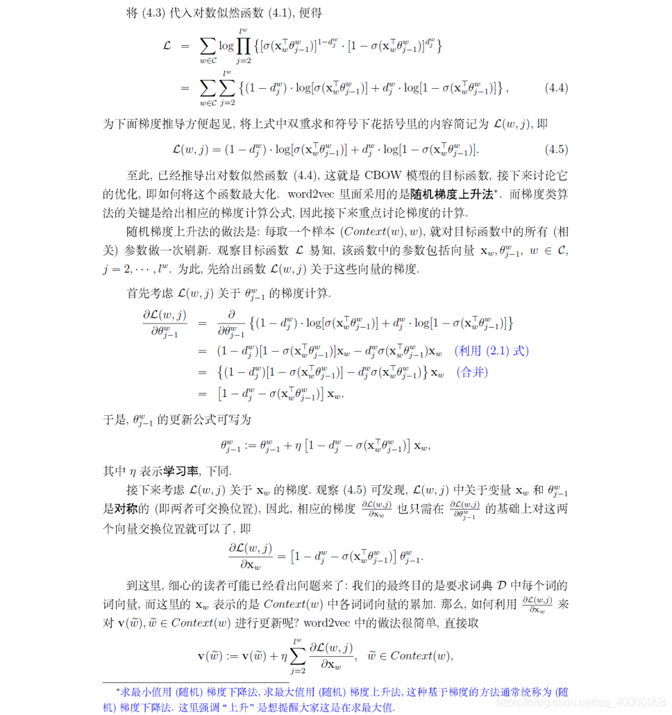
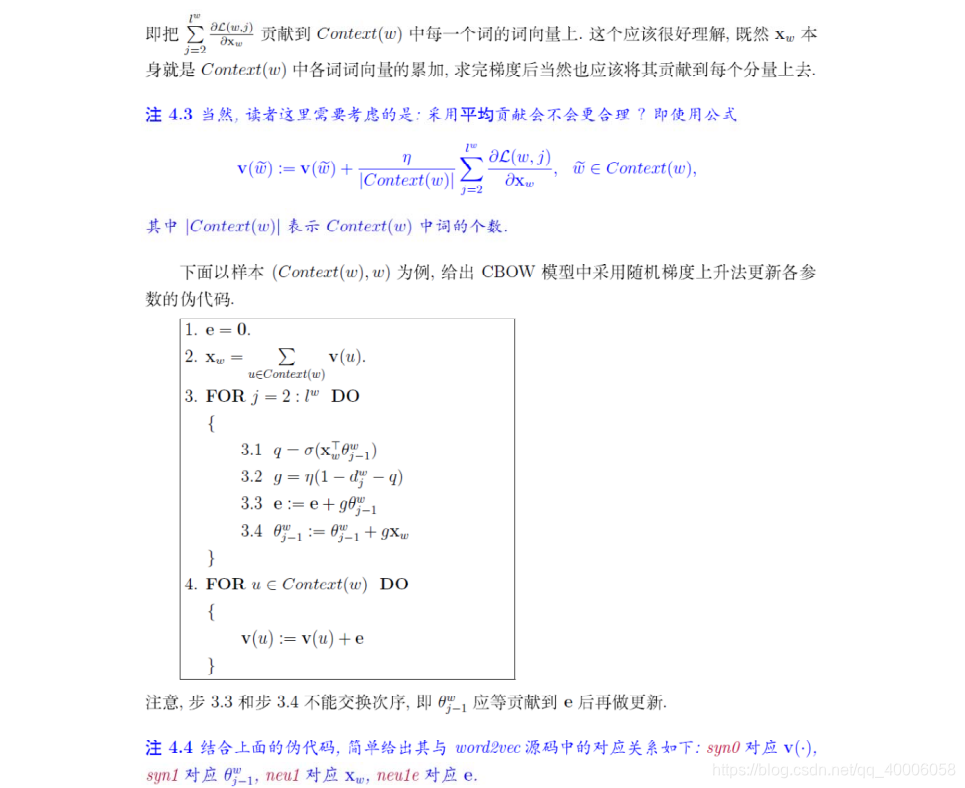
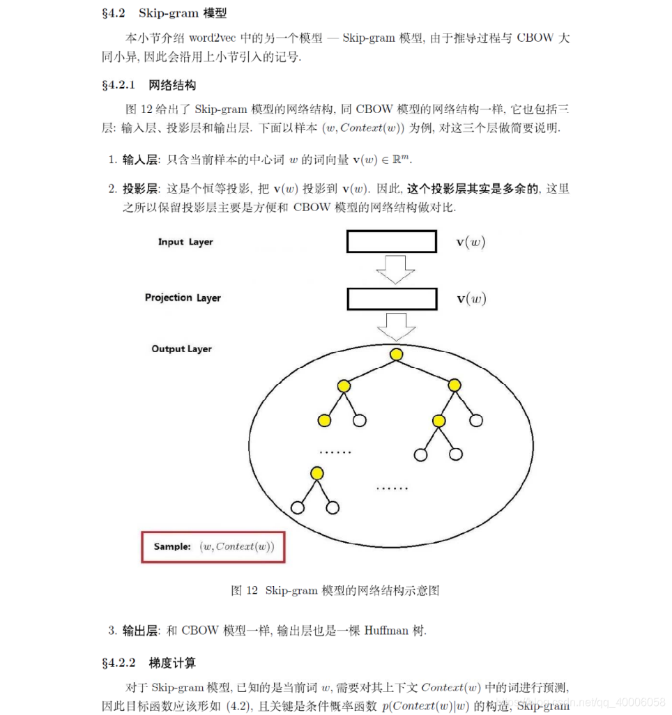
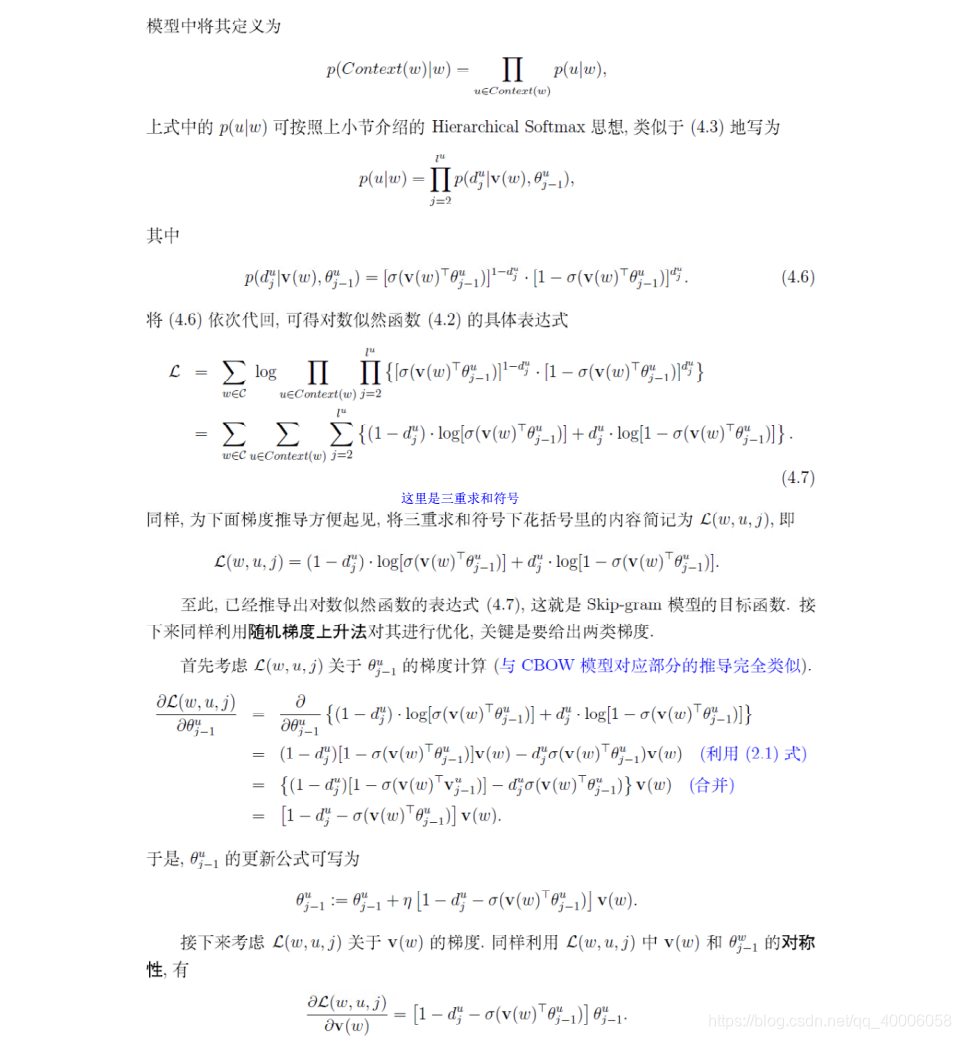
6. 基于Hierarchical Softmax的 skip-gram 和 CBOW 模型数学理论，也很好。