一、概念介绍
自编码器是一种执行数据压缩的网络架构,其中的压缩和解压缩功能是从数据本身学习得到的,而非人为手工设计的。自编码器的两个核心部分是编码器和解码器,它将输入数据压缩到一个潜在表示空间里面,然后再根据这个表示空间将数据进行重构得到最后的输出数据。编码器和解码器都是用神经网络构建的,整个网络的构建方式和普通的神经网络类似,通过最小化输入和输出之间的差异来得到最好的网络。
二、作用
1. 图像去噪;
2. 数据压缩降维。
但是它的图像压缩性能不如JPEG、MP3等传统压缩方法,并且自编码器泛化到其他数据集方面有困难。
三、卷积自编码器实现:
1. 加载数据:
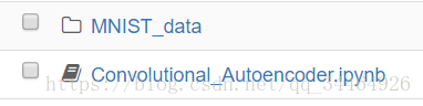
我们的数据基于MNIST数据集,首先需要下载数据并且放在MNIST_data目录下,可以从文章后面提供的链接下载,也可以自行找网上的资源进行下载。目录结构:
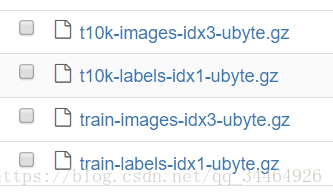
MNIST数据集:
加载数据集:
%matplotlib inline
扫描二维码关注公众号,回复:
2356600 查看本文章

import tensorflow as tf import matplotlib.pyplot as plt from tensorflow.examples.tutorials.mnist import input_data |
2. 数据可视化:
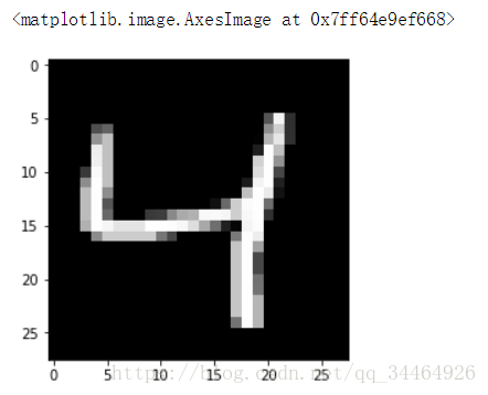
查看一张图片:
| img = mnist.train.images[2] plt.imshow(img.reshape((28, 28)), cmap='Greys_r') |
输出:
3. 构建神经网络结构:
网络的编码器部分将是一个典型的卷积金字塔。每一个卷积层后面都有一个最大池化层来减少维度。解码器需要从一个窄的表示转换成一个宽的重构图像。例如,表示可以是4x4x8 的最大池化层。这是编码器的输出,也是译码器的输入。我们想要从解码器中得到一个28x28x1图像,所以我们需要从狭窄的解码器输入层返回。这是网络的示意图:
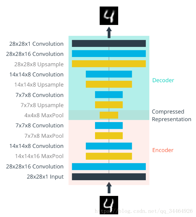
这里我们最后的编码器层有大小4x4x8=128。原始图像的大小为28x28x1=784,因此编码的矢量大约是原始图像大小的16%。这些只是每个层的建议大小。网络的深度和大小都可以更改,但请记住,我们的目标是找到输入数据的一个小表示。
在编码阶段,我们使用卷积层和最大池化层来不断减小输入的维度,在解码器阶段,需要使用反卷积将4x4x8的图片还原到原来的28x28x1。我们使用的这种反卷积方法叫做去卷积,关于反卷积的知识,可以查看这篇文章。在Tensorflow中,很容易使用tf.image.resize_images 或者 tf.image.resize_nearest_neighbor实现。代码如下:
| inputs_ = tf.placeholder(tf.float32, (None, 28, 28, 1), name='inputs') targets_ = tf.placeholder(tf.float32, (None, 28, 28, 1), name='targets') ### 编码器--压缩 conv1 = tf.layers.conv2d(inputs_, 16, (3,3), padding='same', activation=tf.nn.relu) # 当前shape: 28x28x16 maxpool1 = tf.layers.max_pooling2d(conv1, (2,2), (2,2), padding='same') # 当前shape: 14x14x16 conv2 = tf.layers.conv2d(maxpool1, 8, (3,3), padding='same', activation=tf.nn.relu) # 当前shape: 14x14x8 maxpool2 = tf.layers.max_pooling2d(conv2, (2,2), (2,2), padding='same') # 当前shape: 7x7x8 conv3 = tf.layers.conv2d(maxpool2, 8, (3,3), padding='same', activation=tf.nn.relu) # 当前shape: 7x7x8 encoded = tf.layers.max_pooling2d(conv3, (2,2), (2,2), padding='same') # 当前shape: 4x4x8 ### 解码器--还原 upsample1 = tf.image.resize_nearest_neighbor(encoded, (7,7)) # 当前shape: 7x7x8 conv4 = tf.layers.conv2d(upsample1, 8, (3,3), padding='same', activation=tf.nn.relu) # 当前shape: 7x7x8 upsample2 = tf.image.resize_nearest_neighbor(conv4, (14,14)) # 当前shape: 14x14x8 conv5 = tf.layers.conv2d(upsample2, 8, (3,3), padding='same', activation=tf.nn.relu) # 当前shape: 14x14x8 upsample3 = tf.image.resize_nearest_neighbor(conv5, (28,28)) # 当前shape: 28x28x8 conv6 = tf.layers.conv2d(upsample3, 16, (3,3), padding='same', activation=tf.nn.relu) # 当前shape: 28x28x16 logits = tf.layers.conv2d(conv6, 1, (3,3), padding='same', activation=None) #当前shape: 28x28x1 decoded = tf.nn.sigmoid(logits, name='decoded') #计算损失函数 loss = tf.nn.sigmoid_cross_entropy_with_logits(labels=targets_, logits=logits) cost = tf.reduce_mean(loss) #使用adam优化器优化损失函数 opt = tf.train.AdamOptimizer(0.001).minimize(cost) |
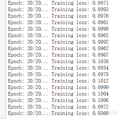
4. 训练网络:
sess = tf.Session() epochs = 20 |
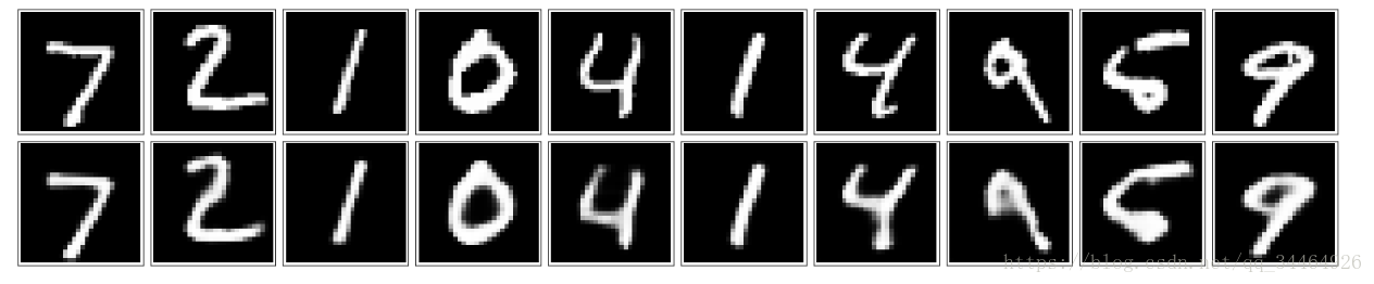
5. matplotlib绘图查看压缩后还原的图片与原图片的区别
四、 使用卷积自编码器进行图像去噪
1. 网络结构:
| inputs_ = tf.placeholder(tf.float32, (None, 28, 28, 1), name='inputs') targets_ = tf.placeholder(tf.float32, (None, 28, 28, 1), name='targets') ### 编码器 conv1 = tf.layers.conv2d(inputs_, 32, (3,3), padding='same', activation=tf.nn.relu) # 当前shape: 28x28x32 maxpool1 = tf.layers.max_pooling2d(conv1, (2,2), (2,2), padding='same') # 当前shape: 14x14x32 conv2 = tf.layers.conv2d(maxpool1, 32, (3,3), padding='same', activation=tf.nn.relu) # 当前shape: 14x14x32 maxpool2 = tf.layers.max_pooling2d(conv2, (2,2), (2,2), padding='same') # 当前shape: 7x7x32 conv3 = tf.layers.conv2d(maxpool2, 16, (3,3), padding='same', activation=tf.nn.relu) # 当前shape: 7x7x16 encoded = tf.layers.max_pooling2d(conv3, (2,2), (2,2), padding='same') # 当前shape: 4x4x16 ### 解码器 upsample1 = tf.image.resize_nearest_neighbor(encoded, (7,7)) # 当前shape: 7x7x16 conv4 = tf.layers.conv2d(upsample1, 16, (3,3), padding='same', activation=tf.nn.relu) # 当前shape: 7x7x16 upsample2 = tf.image.resize_nearest_neighbor(conv4, (14,14)) # 当前shape: 14x14x16 conv5 = tf.layers.conv2d(upsample2, 32, (3,3), padding='same', activation=tf.nn.relu) # 当前shape: 14x14x32 upsample3 = tf.image.resize_nearest_neighbor(conv5, (28,28)) # 当前shape: 28x28x32 conv6 = tf.layers.conv2d(upsample3, 32, (3,3), padding='same', activation=tf.nn.relu) # 当前shape: 28x28x32 logits = tf.layers.conv2d(conv6, 1, (3,3), padding='same', activation=None) #当前shape: 28x28x1 decoded = tf.nn.sigmoid(logits, name='decoded') loss = tf.nn.sigmoid_cross_entropy_with_logits(labels=targets_, logits=logits) cost = tf.reduce_mean(loss) opt = tf.train.AdamOptimizer(0.001).minimize(cost) |
2. 进行100次迭代训练网络(时间更久,建议在GPU上训练):
| sess = tf.Session() epochs = 100 batch_size = 200 # Set's how much noise we're adding to the MNIST images noise_factor = 0.5 sess.run(tf.global_variables_initializer()) for e in range(epochs): for ii in range(mnist.train.num_examples//batch_size): batch = mnist.train.next_batch(batch_size) # Get images from the batch imgs = batch[0].reshape((-1, 28, 28, 1)) # Add random noise to the input images noisy_imgs = imgs + noise_factor * np.random.randn(*imgs.shape) # Clip the images to be between 0 and 1 noisy_imgs = np.clip(noisy_imgs, 0., 1.) # Noisy images as inputs, original images as targets batch_cost, _ = sess.run([cost, opt], feed_dict={inputs_: noisy_imgs, targets_: imgs}) print("Epoch: {}/{}...".format(e+1, epochs), "Training loss: {:.4f}".format(batch_cost)) |
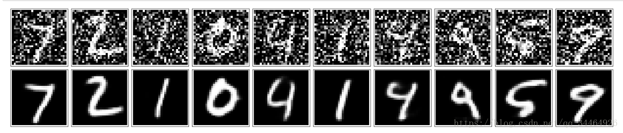
3. 测试网络的去噪效果:
| fig, axes = plt.subplots(nrows=2, ncols=10, sharex=True, sharey=True, figsize=(20,4)) in_imgs = mnist.test.images[:10] noisy_imgs = in_imgs + noise_factor * np.random.randn(*in_imgs.shape) noisy_imgs = np.clip(noisy_imgs, 0., 1.) reconstructed = sess.run(decoded, feed_dict={inputs_: noisy_imgs.reshape((10, 28, 28, 1))}) for images, row in zip([noisy_imgs, reconstructed], axes): for img, ax in zip(images, row): ax.imshow(img.reshape((28, 28)), cmap='Greys_r') ax.get_xaxis().set_visible(False) ax.get_yaxis().set_visible(False) fig.tight_layout(pad=0.1) |
源代码以及数据地址:参见这里