第一周
1.1 监督学习
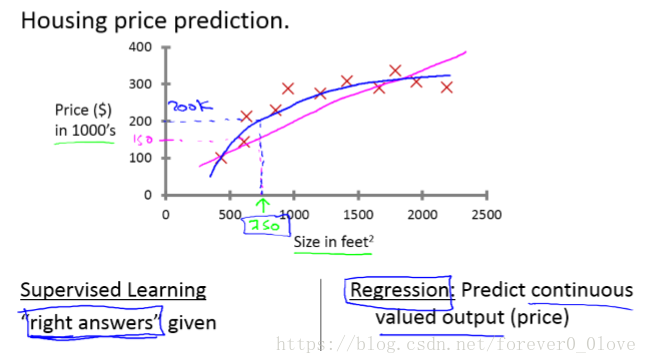
简单地说,监督学习和无监督学习的判别就看输入数据是否有标签(label),有标签的就是监督学习,无标签则就是无监督学习。
监督学习一般用于分类和回归,分类很好理解,就是利用所给数据进行模型训练后再进行分类,类别假设为(0,1,2 ...),而
回归如下图例子所示同样进行训练之后它之后要做的是预测连续的输出值也就是房子的价格。
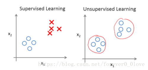
1.2 无监督学习
无监督学习用的最一般的便是聚类,计算机利用数据特征自身学习训练得到训练模型,其数据并没有给出特定答案,也就是所说的标签。
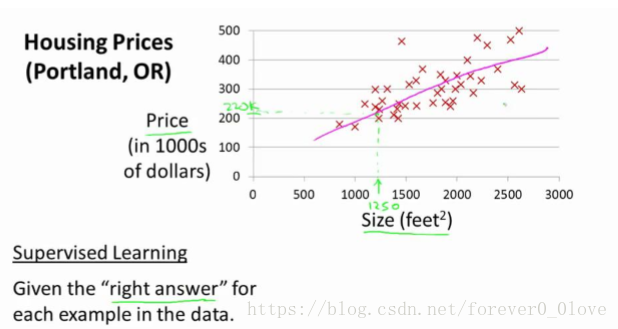
2.1 单变量线性回归(Linear Regression with One Variable)

h是一个从x到y的映射,它代表假设函数,如下图所示,该粉色直线便是我们得到的假设函数,由于其只含有一个特征(输入变量),所以h最有可能是:
plotData实现:
function plotData(x, y)
%PLOTDATA Plots the data points x and y into a new figure
%   PLOTDATA(x,y) plots the data points and gives the figure axes labels of
%   population and profit.
% ====================== YOUR CODE HERE ======================
% Instructions: Plot the training data into a figure using the
%               "figure" and "plot" commands. Set the axes labels using
%               the "xlabel" and "ylabel" commands. Assume the
%               population and revenue data have been passed in
%               as the x and y arguments of this function.
%
% Hint: You can use the 'rx' option with plot to have the markers
%       appear as red crosses. Furthermore, you can make the
%       markers larger by using plot(..., 'rx', 'MarkerSize', 10);

figure; % open a new figure window
plot(x,y,'rx','MarkerSize',10)
ylabel('profit')
xlabel('population')
% ============================================================
end
2.2 代价函数
首先,视频中还是提到这个例子

然后代价函数可以表示为:
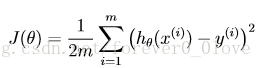
为了便于梯度下降时对代价函数求导消去系数2,便把分母设置为2m,方便计算。
实现代码:
function J = computeCost(X, y, theta)
%COMPUTECOST Compute cost for linear regression
%   J = COMPUTECOST(X, y, theta) computes the cost of using theta as the
%   parameter for linear regression to fit the data points in X and y
% Initialize some useful values
m = length(y); % number of training examples
% You need to return the following variables correctly
J = 0;
% ====================== YOUR CODE HERE ======================
% Instructions: Compute the cost of a particular choice of theta
%               You should set J to the cost.
sum_error = ((X*theta-y)')*(X*theta-y);
J = sum_error/(2*m);
% =========================================================================
end
2.3 梯度下降
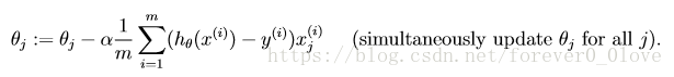
将代价函数分别对两参数求导后更新参数值:
代码:
function [theta, J_history] = gradientDescent(X, y, theta, alpha, num_iters)
%GRADIENTDESCENT Performs gradient descent to learn theta
%   theta = GRADIENTDESENT(X, y, theta, alpha, num_iters) updates theta by
%   taking num_iters gradient steps with learning rate alpha
% Initialize some useful values
m = length(y); % number of training examples
J_history = zeros(num_iters, 1);
for iter = 1:num_iters
    % ====================== YOUR CODE HERE ======================
    % Instructions: Perform a single gradient step on the parameter vector
    %               theta.
    %
    % Hint: While debugging, it can be useful to print out the values
    %       of the cost function (computeCost) and gradient here.
    %
    t_0 = theta(1) - alpha*(1/m)*(((X*theta - y)')*X(:,1));
    t_1 = theta(2) - alpha*(1/m)*(((X*theta - y)')*X(:,2));
    theta(1) = t_0;
    theta(2) = t_1;
    % ============================================================
    % Save the cost J in every iteration
    J_history(iter) = computeCost(X, y, theta);
end
end
这样就实现了参数的更新迭代。
主函数代码:
%% Machine Learning Online Class - Exercise 1: Linear Regression

%  Instructions
%  ------------
%
%  This file contains code that helps you get started on the
%  linear exercise. You will need to complete the following functions
%  in this exericse:
%
%     warmUpExercise.m
%     plotData.m
%     gradientDescent.m
%     computeCost.m
%     gradientDescentMulti.m
%     computeCostMulti.m
%     featureNormalize.m
%     normalEqn.m
%
%  For this exercise, you will not need to change any code in this file,
%  or any other files other than those mentioned above.
%
% x refers to the population size in 10,000s
% y refers to the profit in $10,000s
%
%% Initialization
clear ; close all; clc
%% ==================== Part 1: Basic Function ====================
% Complete warmUpExercise.m
%fprintf('Running warmUpExercise ... \n');
%fprintf('5x5 Identity Matrix: \n');
%warmUpExercise()
%fprintf('Program paused. Press enter to continue.\n');
%pause;
%% ======================= Part 2: Plotting =======================
fprintf('Plotting Data ...\n')
data = load('ex1data1.txt');
X = data(:, 1); y = data(:, 2);
m = length(y); % number of training examples
% Plot Data
% Note: You have to complete the code in plotData.m
plotData(X, y);
fprintf('Program paused. Press enter to continue.\n');
pause;
%% =================== Part 3: Gradient descent ===================
fprintf('Running Gradient Descent ...\n')
X = [ones(m, 1), data(:,1)]; % Add a column of ones to x
theta = zeros(2, 1); % initialize fitting parameters
% Some gradient descent settings
iterations = 1500;
alpha = 0.01;
% compute and display initial cost
computeCost(X, y, theta)
% run gradient descent
theta = gradientDescent(X, y, theta, alpha, iterations);
% print theta to screen
fprintf('Theta found by gradient descent: ');
fprintf('%f %f \n', theta(1), theta(2));
% Plot the linear fit
hold on; % keep previous plot visible
plot(X(:,2), X*theta, '-')
legend('Training data', 'Linear regression')
hold off % don't overlay any more plots on this figure

% Predict values for population sizes of 35,000 and 70,000
predict1 = [1, 3.5] *theta;
fprintf('For population = 35,000, we predict a profit of %f\n',...
    predict1*10000);
predict2 = [1, 7] * theta;
fprintf('For population = 70,000, we predict a profit of %f\n',...
    predict2*10000);
fprintf('Program paused. Press enter to continue.\n');
pause;
%% ============= Part 4: Visualizing J(theta_0, theta_1) =============
fprintf('Visualizing J(theta_0, theta_1) ...\n')
% Grid over which we will calculate J
theta0_vals = linspace(-10, 10, 100);
theta1_vals = linspace(-1, 4, 100);
% initialize J_vals to a matrix of 0's
J_vals = zeros(length(theta0_vals), length(theta1_vals));
% Fill out J_vals
for i = 1:length(theta0_vals)
    for j = 1:length(theta1_vals)
	  t = [theta0_vals(i); theta1_vals(j)];
	  J_vals(i,j) = computeCost(X, y, t);
    end
end
% Because of the way meshgrids work in the surf command, we need to
% transpose J_vals before calling surf, or else the axes will be flipped
J_vals = J_vals';
% Surface plot
figure;
surf(theta0_vals, theta1_vals, J_vals)
xlabel('\theta_0'); ylabel('\theta_1');
% Contour plot
figure;
% Plot J_vals as 15 contours spaced logarithmically between 0.01 and 100
contour(theta0_vals, theta1_vals, J_vals, logspace(-2, 3, 20))
xlabel('\theta_0'); ylabel('\theta_1');
hold on;
plot(theta(1), theta(2), 'rx', 'MarkerSize', 10, 'LineWidth', 2);
练习链接:https://pan.baidu.com/s/115dd47ERAAQfypnLhAAUuA 密码:6ele
实现结果如下:
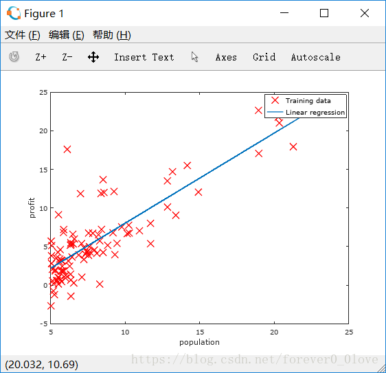
利用plot画的点和最后得到的拟合直线
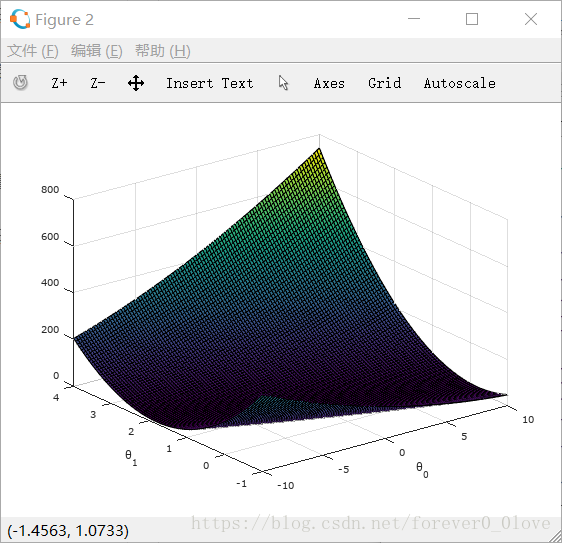
代价函数随着两参数的变化曲面图

迭代完成后最终两参数的坐标值及预测的值。

总体感觉octave跟matlab并没有多大区别,可能是刚用的原因,就当在这上面记笔记吧。。