1、利用sklearn中封装好的房价数据集来实现线性回归。
- 有关线性回归的算法,此处不再详细的赘述,大致说一下思路。首先导入相关的数据集,读取数据
import tensorflow as tf
import numpy as np
from sklearn.datasets import fetch_california_housing
housing = fetch_california_housing(data_home="/Users/a/scikit_learn_data", download_if_missing=True) #下载数据集到指定路径下,如果已下载则不会重复下载
m, n = housing.data.shape #获取数据行数和列数#打印数据集的相关信息
print(m, n)
print(housing.data, housing.target)
print(housing.feature_names) 2.处理数据,给第一列加上全1,保证其输入数据格式的准确
housing_data_plus_bias = np.c_[np.ones((m, 1)), housing.data]3.创建两个常量节点x,y,用来持有数据和标签
x = tf.constant(housing_data_plus_bias, dtype=tf.float32, name='X')
y = tf.constant(housing.target.reshape(-1, 1), dtype=tf.float32, name='y')
4.使用tf框架下的矩阵操作求theta
XT = tf.transpose(x)
theta = tf.matmul(tf.matmul(tf.matrix_inverse(tf.matmul(XT, x)), XT), y)
5.运行创建好的计算图,求出theta值
with tf.Session() as sess:
theta_value = theta.eval() # sess.run(theta)
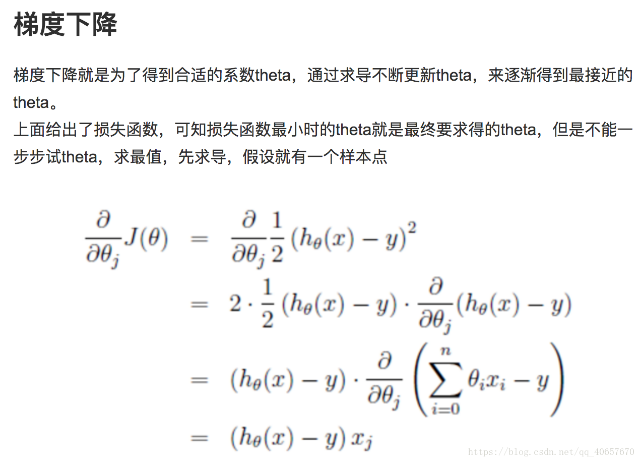
print(theta_value)2、tf实现梯度下降算法,对1-线性回归的改进
1. 处理好数据之后,对其进行归一化操作,目的是更快的进行梯度下降。
import tensorflow as tf
import numpy as np
from sklearn.datasets import fetch_california_housing
from sklearn.preprocessing import StandardScaler


n_epochs = 10000
learning_rate = 0.01

housing = fetch_california_housing(data_home="/Users/a/scikit_learn_data", download_if_missing=True)
m, n = housing.data.shape
housing_data_plus_bias = np.c_[np.ones((m, 1)), housing.data]
scaler = StandardScaler().fit(housing_data_plus_bias)
scaled_housing_data_plus_bias = scaler.transform(housing_data_plus_bias)
X = tf.constant(scaled_housing_data_plus_bias, dtype=tf.float32, name='X')
y = tf.constant(housing.target.reshape(-1, 1), dtype=tf.float32, name='y')2.随机初始化theta
其中random.uniform()表示将数据随机在-1到1之间赋值
theta = tf.Variable(tf.random_uniform([n + 1, 1], -1.0, 1.0), name='theta')3.定义预测值和误差的计算公式,
tf.matual()表示矩阵相乘,回归问题的误差函数使用的是mse,求出误差之后,取其平均值reduce_mean()
y_pred = tf.matmul(X, theta, name="predictions")
error = y_pred - y
mse = tf.reduce_mean(tf.square(error), name="mse")
4.计算梯度
gradients = 2/m * tf.matmul(tf.transpose(X), error)5.更新梯度,tf.assign()函数将后面的值赋给前一个变量
training_op = tf.assign(theta, theta - learning_rate * gradients)
6.设置迭代次数和学习率来计算最终的theta值
init = tf.global_variables_initializer()

with tf.Session() as sess:
    sess.run(init)

    for epoch in range(n_epochs):
        if epoch % 100 == 0:        #每隔100轮打印一次误差
            print("Epoch", epoch, "MSE = ", mse.eval())
        sess.run(training_op)        #运行计算图

    best_theta = theta.eval()
    print(best_theta)
3、使用优化器,对2进行改进
对线性回归算法进行改进,1、使用tf中已经封装好的求梯度的函数 2、有优化器来加快梯度下降的速度。之前的数据处理部分不需要改动,只需将手动计算梯度的部分改成自动求梯度即可。
mse = tf.reduce_mean(tf.square(error), name="mse")
optimizer = tf.train.GradientDescentOptimizer(learning_rate=learning_rate)

training_op = optimizer.minimize(mse)

init = tf.global_variables_initializer()