在实现代码之前,想先再理一下要实现线性回归模型的出发点:
不要迷失,我们的目的是想设计线性回归模型,用来拟合我们得到的数据(本文使用的是二维的数据),所以整个过程重点是要弄清楚,很重要!!!
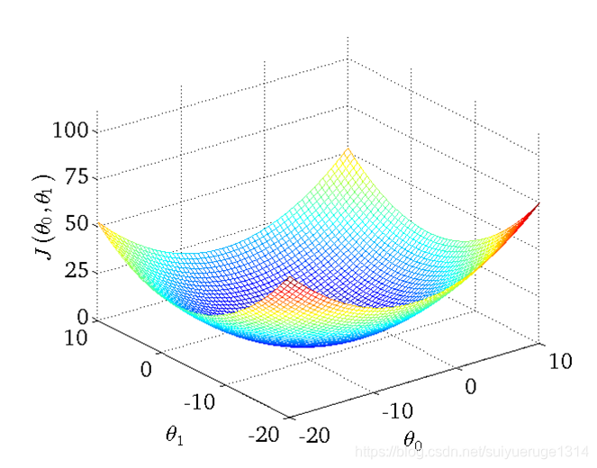
①怎样去衡量模型的好坏?
我们使用Cost Function,对假设的函数进行评价,cost function越小的函数,说明拟合训练数据拟合的越好;而且,注意!我们迭代过程中不是使用全部数据进行优化Cost Function的,而是分批,提高训练速度和收敛速度
更广义而言,深度学习就是在建立极高维模型,使用梯度下降算法的链式法则,在求解损失函数的最小值(准确说是极小值)
②使用什么样的方式来求解模型或者迭代逼近最好模型?
我们使用的是梯度下降算法,但不是唯一方式
建议读一下这篇精彩博客:机器学习入门:线性回归及梯度下降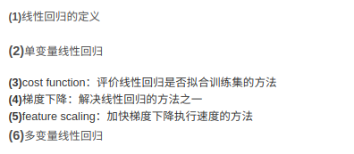
OK,实现!
在了解了线性回归的背景知识之后,现在我们可以动手实现它了。尽管强大的深度学习框架可以减少大量重复性工作,但若过于依赖它提供的便利,会导致我们很难深入理解深度学习是如何工作的。因此,本节将介绍如何只利用Tensor和autograd来实现一个线性回归的训练。
首先,导入本节中实验所需的包或模块,其中的matplotlib包可用于作图,且设置成嵌入显示。

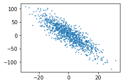
1、生成数据
import tensorflow as tf

print(tf.__version__)

from tensorflow.python.client import device_lib
import os
os.environ['CUDA_VISIBLE_DEVICES'] = "0, 1"
gpus = tf.config.experimental.list_physical_devices(device_type='GPU')
cpus = tf.config.experimental.list_physical_devices(device_type='CPU')
print(gpus, cpus)
# 设置当前程序的可见设备范围
tf.config.experimental.set_visible_devices(devices=gpus, device_type='GPU')

# 设置仅在需要时申请:
for gpu in gpus:
    tf.config.experimental.set_memory_growth(gpu, True)

# 下面的方式是设置Tensorflow固定消耗GPU:0的2GB显存
tf.config.experimental.set_virtual_device_configuration(
    gpus[0],
    [tf.config.experimental.VirtualDeviceConfiguration(memory_limit=200)]
)

def get_available_gpus():
  local_device_protos = device_lib.list_local_devices()
  return [x.name for x in local_device_protos if x.device_type == 'GPU']

print(get_available_gpus())

# 生成数据
with tf.device('/device:GPU:0'):
    w = tf.constant([[2, -3.4]])
    b = tf.constant([4.2])
    x = tf.random.normal([1000, 2], mean=0, stddev=10)
    e = tf.random.normal([1000, 2], mean=0, stddev=0.1)
    W = tf.Variable(tf.constant([5, 1]))
    B = tf.Variable(tf.constant([1]))

import random
from matplotlib import pyplot as plt
# 线性回归模型, y =
# 生成数据,生成1000组数据

num_inputs = 2
num_examples = 1000
true_y = tf.matmul(x, tf.transpose(w)) + b
x, true_y

def set_figsize(figsize=(3.5, 2.5)):
    plt.rcParams['figure.figsize'] = figsize

set_figsize()
plt.scatter(x[: ,1], true_y, 1)
2、读取数据
def process(x, y):
    return x, y

db = tf.data.Dataset.from_tensor_slices((x, true_y))
db = db.shuffle(100)
db2 = db.map(process)
db_batch = db.batch(32)
db_iter = next(iter(db_batch))
# 查看一组数据,使用next方法迭代一组
print(db_iter[1].shape)
3、初始化模型参数和构建模型
class Mymodel():
    def __init__(self):
        self.w = tf.Variable([[2.3, 1.2]])
        self.b = tf.Variable([3.0])

    def __call__(self, x):
        self.y = tf.matmul(x , tf.transpose(self.w)) + self.b
        return self.y
4、定义损失函数
def loss(predicted_y, desired_y):
    return tf.reduce_mean(tf.square(predicted_y - tf.reshape(desired_y, predicted_y.shape)))
5、定义优化算法
def train(model, inputs, outputs, learning_rate):
    with tf.GradientTape() as t:
        current_loss = loss(model(inputs), outputs)
        print('loss',current_loss)
    dW, db = t.gradient(current_loss, [model.w, model.b])
    # tf.assign_sub(ref, value, use_locking=None, name=None),变量 ref 减去 value值,即 ref = ref - value
    model.w.assign_sub(learning_rate * dW)
    model.b.assign_sub(learning_rate * db)
6、训练模型
model = Mymodel()

Ws, bs = [], []
epoches = 100

steps = int(1000/32)
for i in range(epoches):
    for d in iter(db_batch):
#         d = next(iter(db_batch))
        it = d[0]
#         print(it)
        ot = d[1]
#         print(ot)
#         current_loss = loss(model(it), ot)
#         print(current_loss)

        train(model, it, ot, learning_rate=0.001)

    Ws.append(model.w.numpy())
    bs.append(model.b.numpy())
    print('w',(Ws[-1]))
    print('b',(bs[-1]))
#         print('Epoch %2d: W=%1.2f b=%1.2f, loss=%2.5f' %
#               (epoch, Ws[-1], bs[-1], current_loss))
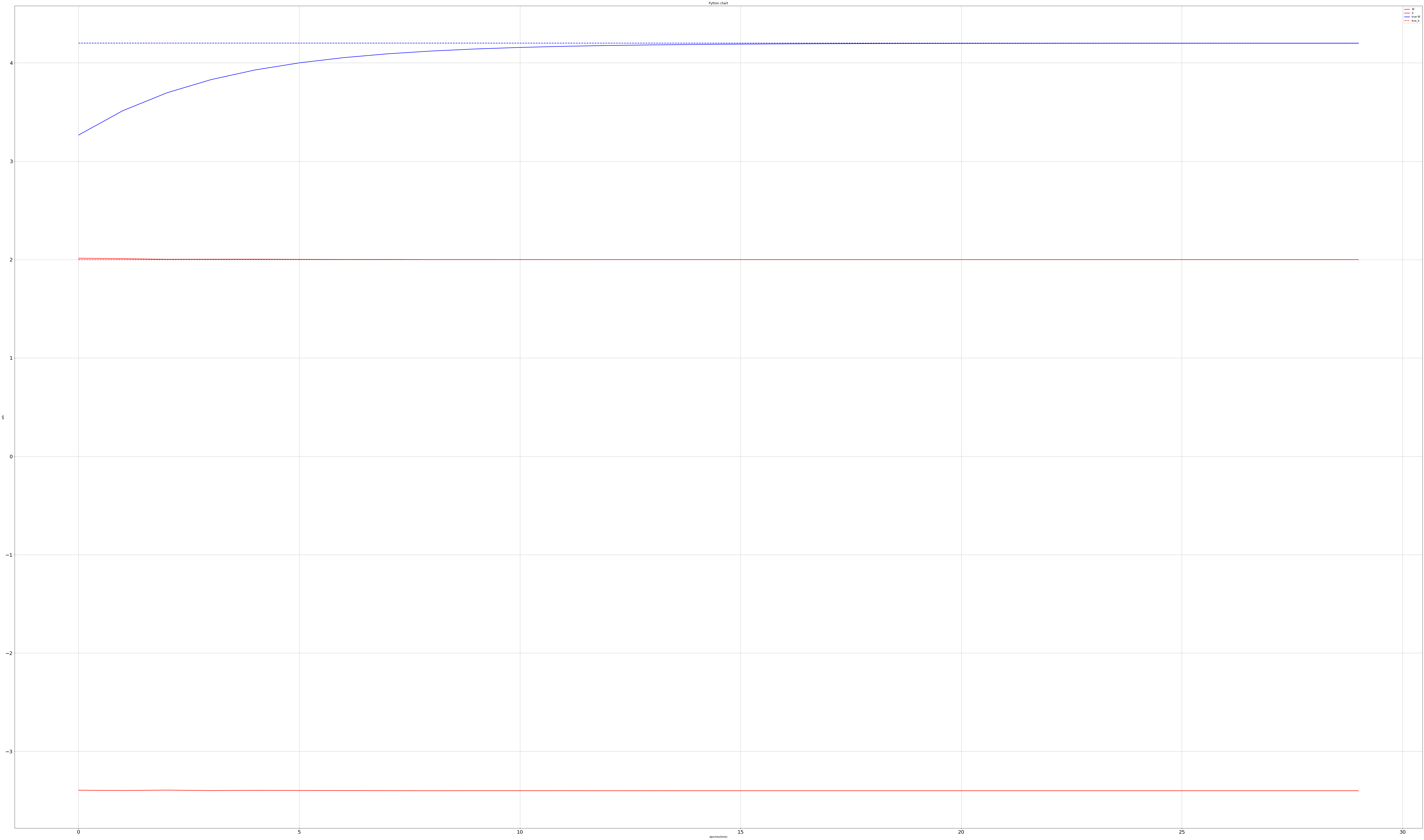
7、作训练权重收敛图
plt.figure(figsize=(100, 60))
plt.plot(range(epoches), [i[0] for i in Ws], 'r',
         range(epoches), [i[0] for i in bs], 'b', linewidth=2)
plt.plot([2] * epoches, 'r--',
         [4.2] * epoches, 'b--', linewidth=2)

plt.xlabel('epoches(time)')
plt.ylabel("w/b")
plt.grid(True)
plt.title("Python chart")
plt.xticks(fontsize=20)
plt.yticks(fontsize=20)
plt.legend(['W', 'b', 'true W', 'true_b'])
plt.show()