本文是Google机器学习教程(ML Crash Course with TensorFlow APIs)的学习笔记。教程地址:
https://developers.google.com/machine-learning/crash-course/ml-intro
6. First Steps with TensorFlow
代码及解说地址:
https://colab.research.google.com/notebooks/mlcc/first_steps_with_tensor_flow.ipynb
########################################################Setup

import math

from IPython import display
from matplotlib import cm
from matplotlib import gridspec
from matplotlib import pyplot as plt
import numpy as np
import pandas as pd
from sklearn import metrics
import tensorflow as tf
from tensorflow.python.data import Dataset

tf.logging.set_verbosity(tf.logging.ERROR)
pd.options.display.max_rows = 10
pd.options.display.float_format = '{:.1f}'.format
# 加载数据,封装到pandas Dataframe中
california_housing_dataframe = pd.read_csv("https://storage.googleapis.com/mledu-datasets/california_housing_train.csv", sep=",")
#数据随机排序,这样保障的SGD效果
california_housing_dataframe = california_housing_dataframe.reindex(
np.random.permutation(california_housing_dataframe.index))
#为了方便处理数据,将房价数据缩小1000倍
california_housing_dataframe["median_house_value"] /= 1000.0随机排序及缩放后的数据:

#对数据有个整体统计分析
california_housing_dataframe.describe()
# 首先选取total_rooms为特征
my_feature = california_housing_dataframe[["total_rooms"]]

# total_room的样本数据都是数字,因此定义为tf的数字类型特征列
feature_columns = [tf.feature_column.numeric_column("total_rooms")]

# 目标是median_house_value
targets = california_housing_dataframe["median_house_value"]
feature_columns:
![]()
# 定义优化为梯度下降,学习效率为0.0000001,这个学习很低,可以逐步提高来优化模型
my_optimizer=tf.train.GradientDescentOptimizer(learning_rate=0.0000001)
# 梯度裁剪确保了梯度的大小在训练期间不会变得太大,从而导致梯度下降失败。
my_optimizer = tf.contrib.estimator.clip_gradients_by_norm(my_optimizer, 5.0)

# 定义线性回归,将前面定义的特征列和优化方法作为参数
linear_regressor = tf.estimator.LinearRegressor(
    feature_columns=feature_columns,
    optimizer=my_optimizer
)
接下来是定义数据输入函数,该函数是将pd获取的数据组织成tf学习使用的dataset:
def my_input_fn(features, targets, batch_size=1, shuffle=True, num_epochs=None):
    """用一个特征来训练线性回归模型

    参数:
      features: pandas DataFrame 格式的特征数据
      targets: pandas DataFrame 格式的目标值(标签)
      batch_size: 模型训练的批次大小
      shuffle: True / False. 是否要将数据重新洗牌
      num_epochs: 数据重复次数. None = 无限重复
    返回:
      下一个数据批次构成的元组(features, labels)
    """

    # 将pandas DataFrame数据转换成np arrays的字典类型. 结果: {'total_rooms': array([1410., 2046., 2987., ..., 2478., 9882., 1923.])}
    features = {key: np.array(value) for key, value in dict(features).items()}

    # 构建tf的dataset,设置batching/repeating
    ds = Dataset.from_tensor_slices((features, targets))  # warning: 2GB limit
    ds = ds.batch(batch_size).repeat(num_epochs)

    # 根据需要重新洗牌数据
    if shuffle:
        ds = ds.shuffle(buffer_size=10000)#洗牌的样本大小

    # 获取下一个数据批次的features/labels
    features, labels = ds.make_one_shot_iterator().get_next()
    return features, labels
训练模型:
_ = linear_regressor.train(
    input_fn = lambda:my_input_fn(my_feature, targets),
    steps=100
)
评估训练后的模型:
# 创建预测的输入函数,每次预测一个样本,所以不需要循环和洗牌:num_epochs=1, shuffle=False
prediction_input_fn =lambda: my_input_fn(my_feature, targets, num_epochs=1, shuffle=False)

# 用训练的模型来预测
predictions = linear_regressor.predict(input_fn=prediction_input_fn)

# 讲预测结果转换成NumPy array, 方便度量误差
predictions = np.array([item['predictions'][0] for item in predictions])

# 计算均方误差MSE和均方根误差RMSE
mean_squared_error = metrics.mean_squared_error(predictions, targets)
root_mean_squared_error = math.sqrt(mean_squared_error)

# 计算样本的最大、最小及范围
min_house_value = california_housing_dataframe["median_house_value"].min()
max_house_value = california_housing_dataframe["median_house_value"].max()
min_max_difference = max_house_value - min_house_value

print("Min. Median House Value: %0.3f" % min_house_value)
print("Max. Median House Value: %0.3f" % max_house_value)
print("Difference between Min. and Max.: %0.3f" % min_max_difference)
print("Root Mean Squared Error: %0.3f" % root_mean_squared_error)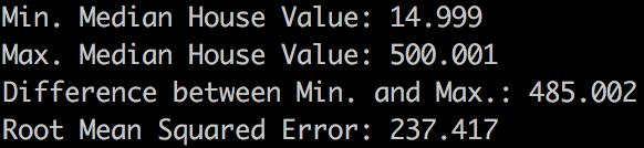
可以看到目前模型效果很糟糕,RMSE很大,几乎到了样本区间的一半。
思考下将模型训练的更好?
可以先看看自己的预测与样本之间的偏差:
calibration_data = pd.DataFrame()
calibration_data["predictions"] = pd.Series(predictions)
calibration_data["targets"] = pd.Series(targets)
calibration_data.describe()
这些数字也体现了我们的模型目前很糟糕。
还可以通过绘制图形来看看我们的模型效果如何(因为目前是一个特征,所以可以绘制二维图形):
# 选择300个样本进行绘图分析
sample = california_housing_dataframe.sample(n=300)

# 获得样本中特征最大最小值
x_0 = sample["total_rooms"].min()
x_1 = sample["total_rooms"].max()

# 获取模型训练后的权重与偏差
weight = linear_regressor.get_variable_value('linear/linear_model/total_rooms/weights')[0]
bias = linear_regressor.get_variable_value('linear/linear_model/bias_weights')

# 计算最大、最小特征值时的预测值
y_0 = weight * x_0 + bias
y_1 = weight * x_1 + bias

# 绘制最大最小点之间的直线,这就是目前我们的模型几何表示
plt.plot([x_0, x_1], [y_0, y_1], c='r')

# 绘制图形坐标轴标签
plt.ylabel("median_house_value")
plt.xlabel("total_rooms")

# 将样本绘制到图形上(x-特征值,y-标签)
plt.scatter(sample["total_rooms"], sample["median_house_value"])

# 显示图形
plt.show()
可以看到,模型(红线)与样本(蓝点)拟合的很差。
将学习效率提高到0.001,效果会好一些:


通过图形也可以清晰的看到,单个特征是不能得到很好的预测模型的。
最后,将前面模型的代码组合到一个函数中:
def train_model(learning_rate, steps, batch_size, input_feature):
    """Trains a linear regression model.

    Args:
      learning_rate: A `float`, the learning rate.
      steps: A non-zero `int`, the total number of training steps. A training step
        consists of a forward and backward pass using a single batch.
      batch_size: A non-zero `int`, the batch size.
      input_feature: A `string` specifying a column from `california_housing_dataframe`
        to use as input feature.

    Returns:
      A Pandas `DataFrame` containing targets and the corresponding predictions done
      after training the model.
    """

    periods = 10
    steps_per_period = steps / periods

    my_feature = input_feature
    my_feature_data = california_housing_dataframe[[my_feature]].astype('float32')
    my_label = "median_house_value"
    targets = california_housing_dataframe[my_label].astype('float32')

    # Create input functions.
    training_input_fn = lambda: my_input_fn(my_feature_data, targets, batch_size=batch_size)
    predict_training_input_fn = lambda: my_input_fn(my_feature_data, targets, num_epochs=1, shuffle=False)

    # Create feature columns.
    feature_columns = [tf.feature_column.numeric_column(my_feature)]

    # Create a linear regressor object.
    my_optimizer = tf.train.GradientDescentOptimizer(learning_rate=learning_rate)
    my_optimizer = tf.contrib.estimator.clip_gradients_by_norm(my_optimizer, 5.0)
    linear_regressor = tf.estimator.LinearRegressor(
        feature_columns=feature_columns,
        optimizer=my_optimizer
    )

    # Set up to plot the state of our model's line each period.
    plt.figure(figsize=(15, 6))
    plt.subplot(1, 2, 1)
    plt.title("Learned Line by Period")
    plt.ylabel(my_label)
    plt.xlabel(my_feature)
    sample = california_housing_dataframe.sample(n=300)
    plt.scatter(sample[my_feature], sample[my_label])
    colors = [cm.coolwarm(x) for x in np.linspace(-1, 1, periods)]

    # Train the model, but do so inside a loop so that we can periodically assess
    # loss metrics.
    print("Training model...")
    print("RMSE (on training data):")
    root_mean_squared_errors = []
    for period in range(0, periods):
        # Train the model, starting from the prior state.
        linear_regressor.train(
            input_fn=training_input_fn,
            steps=steps_per_period,
        )
        # Take a break and compute predictions.
        predictions = linear_regressor.predict(input_fn=predict_training_input_fn)
        predictions = np.array([item['predictions'][0] for item in predictions])

        # Compute loss.
        root_mean_squared_error = math.sqrt(
            metrics.mean_squared_error(predictions, targets))
        # Occasionally print the current loss.
        print("  period %02d : %0.2f" % (period, root_mean_squared_error))
        # Add the loss metrics from this period to our list.
        root_mean_squared_errors.append(root_mean_squared_error)
        # Finally, track the weights and biases over time.
        # Apply some math to ensure that the data and line are plotted neatly.
        y_extents = np.array([0, sample[my_label].max()])

        weight = linear_regressor.get_variable_value('linear/linear_model/%s/weights' % input_feature)[0]
        bias = linear_regressor.get_variable_value('linear/linear_model/bias_weights')

        x_extents = (y_extents - bias) / weight
        x_extents = np.maximum(np.minimum(x_extents,
                                          sample[my_feature].max()),
                               sample[my_feature].min())
        y_extents = weight * x_extents + bias
        plt.plot(x_extents, y_extents, color=colors[period])
    print("Model training finished.")

    # Output a graph of loss metrics over periods.
    plt.subplot(1, 2, 2)
    plt.ylabel('RMSE')
    plt.xlabel('Periods')
    plt.title("Root Mean Squared Error vs. Periods")
    plt.tight_layout()
    plt.plot(root_mean_squared_errors)

    # Create a table with calibration data.
    calibration_data = pd.DataFrame()
    calibration_data["predictions"] = pd.Series(predictions)
    calibration_data["targets"] = pd.Series(targets)
    display.display(calibration_data.describe())

    print("Final RMSE (on training data): %0.2f" % root_mean_squared_error)

    return calibration_data
7. 组合特征和离群值Synthetic Features and Outliers
组合特征能够减少特征数量,计算一个特征就能同时引入多个特征,提高模型的效率;排除离群值可以提高模型的精确度;
增加一个特征rooms_per_person,该特征是其他特征计算来的:total_rooms / population,用新特征训练模型:
california_housing_dataframe["rooms_per_person"] = (
    california_housing_dataframe["total_rooms"] / california_housing_dataframe["population"])

calibration_data = train_model(
    learning_rate=0.05,
    steps=500,
    batch_size=5,
    input_feature="rooms_per_person")

可以看到模型最后一次训练RMSE反而增大了,表示超过了梯度的最低点,学习效率要适当减小(当前是0.05)
接下来处理离群值,通过绘制样本数据的图形来分析离群值:
#分析离群值
plt.figure(figsize=(15, 6))
plt.subplot(1, 2, 1)
#绘制预测值(x)与标签值(y)的散点图
plt.scatter(calibration_data["predictions"], calibration_data["targets"])

plt.subplot(1, 2, 2)
#绘制特征值rooms_per_person的直方分布图
_ = california_housing_dataframe["rooms_per_person"].hist()

plt.show()
可以看到离群值的分布状况,左边是预测值(x)与目标值(y);右边是rooms_per_person的直方图分布,大部分数据在0-5之间,所以大于5的可以过滤掉。
排除离群值:
# 排除离群值
california_housing_dataframe["rooms_per_person"] = (
    california_housing_dataframe["rooms_per_person"]).apply(lambda x: min(x, 5))
# 绘制特征值rooms_per_person的直方分布图,看到大于5的利群值已经被排除
_ = california_housing_dataframe["rooms_per_person"].hist()

# 重新训练模型
calibration_data = train_model(
    learning_rate=0.05,
    steps=500,
    batch_size=5,
    input_feature="rooms_per_person")
# 绘制预测值(x)与标签值(y)的散点图
_ = plt.scatter(calibration_data["predictions"], calibration_data["targets"])
可以看到只有0-5之间的特征值了。
排除离散值后的训练结果:
