Tensorflow学习（一）--使用TensorFlow实现线性回归

本博客仅为作者记录笔记之用，不免有很多细节不对之处。还望各位看官能够见谅，欢迎批评指正。

最近发现自己都没有真正好好学习过TensorFlow，只是看看别人project的代码，然后能跑起来就行，实际自己想要去搭建一些网络还是很困难，因此准备写一个使用TensorFlow实现一些网络的系列。这是第一篇，因此就从最简单的线性回归开始。

首先简单介绍一下线性回归。线性回归的表达式为：

y=wx+b $y=wx+b$
其中w为权重，b为偏移量。
定义线性回归的损失函数：

loss=1n−1∑ni=1(y^−y)2 $loss={1\over n-1}\sum_{i=1}^n(\hat{y}-y)^2$
主要是通过梯度下降法，不断的去更新权重w，b，来最小化损失函数。

首先我们需要导入TensorFlow、numpy以及matplotlib这三个库

import tensorflow as tf
import numpy as np
import matplotlib.pyplot as plt
rng = np.random

设置模型的参数，定义学习率、模型的迭代次数以及迭代多少次计算一次模型损失

# Parameters
learning_rate = 0.01
training_epochs = 5000
display_step = 50

定义输入数据 X , Y以及样本个数n

# Training Data
train_X = np.asarray([3.3, 4.4, 5.5, 6.71, 6.93, 4.168, 9.779, 6.182, 7.59, 2.167,
                      7.042, 10.791, 5.313, 7.997, 5.654, 9.27, 3.1])
train_Y = np.asarray([1.7, 2.76, 2.09, 3.19, 1.694, 1.573, 3.366, 2.596, 2.53, 1.221,
                      2.827, 3.465, 1.65, 2.904, 2.42, 2.94, 1.3])
n_samples = train_X.shape[0]

初始化模型的输入输出变量以及定义模型的权重系数和偏移量

# tf Graph Input
X = tf.placeholder(tf.float32)
Y = tf.placeholder(tf.float32)

# Set model weights
W = tf.Variable(rng.randn(), name="weight")
b = tf.Variable(rng.randn(), name="bias")

定义线性模型，使用均方误差作为模型的训练误差。优化训练误差的方法为梯度下降

# Construct a linear model
pred = tf.add(tf.multiply(X, W), b)

# Mean squared error
cost = tf.reduce_sum(tf.pow(pred-Y, 2))/(2*n_samples)
# Gradient descent
#  Note, minimize() knows to modify W and b because Variable objects are trainable=True by default
optimizer = tf.train.GradientDescentOptimizer(learning_rate).minimize(cost)

# Initialize the variables (i.e. assign their default value)
init = tf.global_variables_initializer()

准备工作都做好之后，我们就可以开始进行训练线性模型了。

# 开始训练
with tf.Session() as sess:

    # 执行初始化操作
    sess.run(init)

    # 拟合模型数据
    for epoch in range(training_epochs):
        for (x, y) in zip(train_X, train_Y):
            sess.run(optimizer, feed_dict={X: x, Y: y})

        # 每50次迭代后在控制台输出模型当前训练的loss以及权重大小
        if (epoch+1) % display_step == 0:
            c = sess.run(cost, feed_dict={X: train_X, Y:train_Y})
            print("Epoch:", '%04d' % (epoch+1), "cost=", "{:.9f}".format(c), \
                "W=", sess.run(W), "b=", sess.run(b))

    print("Optimization Finished!")
    training_cost = sess.run(cost, feed_dict={X: train_X, Y: train_Y})
    print("Training cost=", training_cost, "W=", sess.run(W), "b=", sess.run(b), '\n')

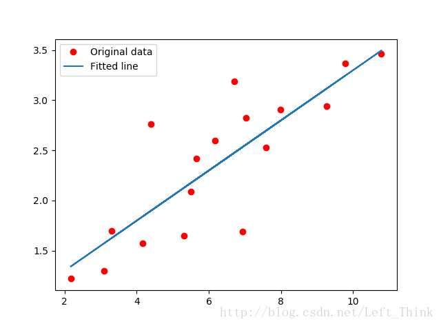
    # 画出拟合图像
    plt.plot(train_X, train_Y, 'ro', label='Original data')
    plt.plot(train_X, sess.run(W) * train_X + sess.run(b), label='Fitted line')
    plt.legend()
    plt.show()

得到最后的模型损失和参数值

画出拟合直线与数据点的图如下所示：
这里写图片描述

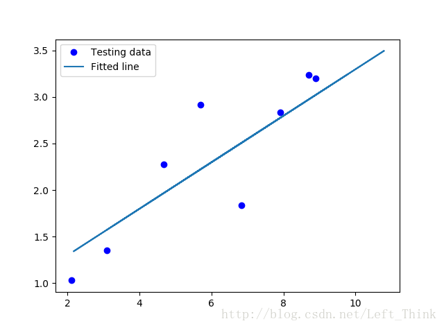
得到模型之后，我们将模型在测试数据上进行测试。

    # 创建测试数据
    test_X = np.asarray([6.83, 4.668, 8.9, 7.91, 5.7, 8.7, 3.1, 2.1])
    test_Y = np.asarray([1.84, 2.273, 3.2, 2.831, 2.92, 3.24, 1.35, 1.03])

    print("Testing... (Mean square loss Comparison)")
    testing_cost = sess.run(
        tf.reduce_sum(tf.pow(pred - Y, 2)) / (2 * test_X.shape[0]),
        feed_dict={X: test_X, Y: test_Y})  # same function as cost above
    print("Testing cost=", testing_cost)
    print("Absolute mean square loss difference:", abs(
        training_cost - testing_cost))

    plt.plot(test_X, test_Y, 'bo', label='Testing data')
    plt.plot(train_X, sess.run(W) * train_X + sess.run(b), label='Fitted line')
    plt.legend()
    plt.show()

得到图像如下所示：

最后附上实现完整代码的GitHub仓库，欢迎各位看官star和fork~~~~

Tensorflow学习（一）--使用TensorFlow实现线性回归

猜你喜欢