Logistic Regression是一个经典的判别学习分类方法。参考资料—西瓜书&&机器学习公开课-Andrew Ng。
首先我们来看为什么Logistic Regression被称为对数几率回归。
几率:将一个实例映射到正例或者负例的可能性比率。令
表示将样本分类成正例的概率。那么
就表示将样本分类成负例的概率。那么这里的几率表示为:
对数几率:对数几率就是对上式求对数。
回归就是线性回归方法。因此:对数几率回归的表达式如下:
。
经过简单的代数运算,我们得到
;以及
。
我们看到 和 的表达式实际上就是Sigmoid函数。那么为什么要这样做呢?
通过线性回归的方法做分类,理想的情况下是这样来做:
令
,当z<0,样本被分类成负例;当z>0,样本被分类成正例;当z=0,样本可以任意分类。显然,这里预测函数为单位阶跃函数
g(z)的函数图像如下图红线所示:
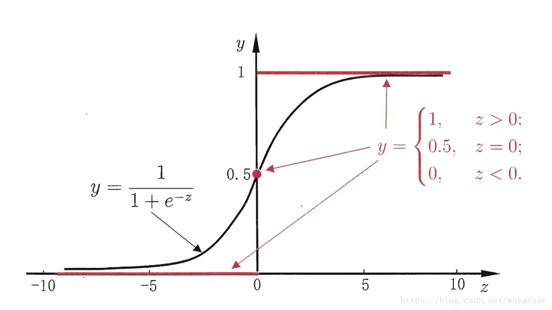
而单位阶跃函数是不连续不可微的,这对于我们求解参数带来了很大的不便。
因此,科学家们就想到用另外一个连续可微函数近似替代这个阶跃函数。常用的替代函数如上图黑线所示,它也被称为Sigmoid函数,也可以被称为对数几率函数。同样地,当对数几率函数值大于0.5,样本被分类成正例;小于0.5,样本被分类成负例;等于0.5,样本可被任意分类。
上面就是对对数几率函数的一些解释。咱们继续,在得到了 和 之后,我们得到后验概率如下,对某一个训练样本:
。
写出对数似然函数:
。
诶 忽然发现有些不对,
不好处理。于是,我们改写:
。
于是,
。
极大化对数似然等价于极小化其负数
。
从损失函数的角度也可以导出上述式子
定义损失函数
化简得到 ,
训练数据总体损失
。
最终目标为
目标函数对
求偏导可得
。
这个式子的解析解不容易给出,于是利用标准梯度下降法给出
的迭代公式如下:
。
当然,也可以通过牛顿法,随机梯度下降等其他经典的方法求解。
下面附上代码(Python实现),建议在PyCharm下运行,数据集采用的是《机器学习实战》的Logistic回归测试数据:
# -*- coding:utf-8 -*-
# This class is built for logistic regression
__author__ = 'yanxue'

import numpy as np
from numpy import random
from numpy import linalg
from matplotlib import pyplot as plt
import math

class LogisticRegression:
    def __init__(self):
        pass

    def learning(self, data, label, learning_rate=0.1, convergence_rate=1):
        """Learning process of the logistic regression"""
        n, d = data.shape
        self.theta = random.randn(d + 1)
        theta0 = random.randn(d + 1)
        count = 0
        c_error = 0
        for j, x in enumerate(data):
            pLabel = lr.classify(x)
            c_error += pLabel != label[j]
        yield c_error, theta0
        ind = 0
        while linalg.norm(theta0 - self.theta) > convergence_rate:
            print('theta_{} = {}'.format(count, theta0))
            self.theta = theta0.copy()
            # gradient decent
            theta0 -= learning_rate * sum(map(self.__fun, [(data[i], label[i]) for i in range(n)]))
            # Stochastic gradient descent
            # theta0 -= learning_rate * self.__fun((data[ind % n], label[ind % n]))
            # ind += 1
            # Batch gradient descent
            # theta0 -= learning_rate * sum(map(self.__fun, [(data[i % n], label[i % n]) for i in range(ind, ind + 10)]))
            # ind += 10
            c_error = 0
            for j, x in enumerate(data):
                pLabel = lr.classify(x)
                c_error += pLabel != label[j]
            yield c_error, self.theta
            count += 1

    def __fun(self, trainx):
        return -trainx[1] * np.append(trainx[0], 1) + np.append(trainx[0], 1) * self.s(trainx[0])

    def classify(self, x):
        if self.s(x) < 0.5:
            return 0
        elif self.s(x) >= 0.5:
            return 1

    def s(self, inx):
        """Sigmoid function value"""
        try:
            re = 1 / (1 + math.exp(-np.dot(self.theta, np.append(inx, 1))))
        except OverflowError as e:
            print(e)
            re = 1
        return re

    def __str__(self):
        return "Logistic regression"

trainData = np.loadtxt('data/LogisticRegressionTestSet.txt', delimiter='\t')
trainX = trainData[:, [0, 1]]
trainY = trainData[:, 2]
lr = LogisticRegression()
# ------ Plot the data points ------
x1 = np.arange(-4.0, 3.2, 0.1)
plt.close()
plt.ion()  #interactive mode on
fig = plt.figure()
ax = fig.add_subplot(1, 1, 1)
# ------ End of plot ------
for c_error, c_theta in lr.learning(trainX, trainY):
    # ------ Plot the iterative process ------
    plt.grid()
    plt.scatter(trainX[trainY == 0, 0], trainX[trainY == 0, 1], c='r')  # plot positive instances
    plt.scatter(trainX[trainY == 1, 0], trainX[trainY == 1, 1], c='b')  # plot negative instances
    plt.xlabel('$x_1$')
    plt.ylabel('$x_2$')
    plt.title('Logistic Regression Demo')
    x2 = (-c_theta[0] * x1 - c_theta[2]) / c_theta[1]
    plt.plot(x1, x2)
    plt.text(-4, 12.5, 'errorNum = {}'.format(c_error))
    # ------ End of plot ------
    plt.pause(0.2)