scipy1.1.0版本的接口有很大,变化,也新增了函数。使用scipy求解微分方程主要使用scipy.integrate模块,函数是odeint,solve_ivp(初值问题),可以求解一阶、二阶以及高阶方程或方程组。
下面直接上代码,已有详细注释
'''
使用scipy求解微分方程,包括一阶、二阶和高阶微分方程
从scipy1.1.0版本开始,相关的求解函数API变化比较大,也新增了一些函数
scipy求解微分方程的函数主要有:
(1) scipy.integrate.odeint(func, y0, t, args=(), Dfun=None, col_deriv=0, full_output=0, ml=None, mu=None, rtol=None, atol=None, tcrit=None, h0=0.0, hmax=0.0, hmin=0.0, ixpr=0, mxstep=0, mxhnil=0, mxordn=12, mxords=5, printmessg=0, tfirst=False)
Solve a system of ordinary differential equations using lsoda from the FORTRAN library odepack.
Solves the initial value problem for stiff or non-stiff systems of first order ode-s:
dy/dt = func(y, t, ...) [or func(t, y, ...)]
where y can be a vector.
在scipy1.1.0版本中odeint引进tfirst参数,其值为True时,func的参数顺序为 t,y;
(2) scipy.integrate.solve_ivp(fun, t_span, y0, method='RK45', t_eval=None, dense_output=False, events=None, vectorized=False, **options)[source]
官网推荐在新代码中使用第二个函数,对于此函数主要注意两个参数:t_span和t_eval,t_span是(t0,tf)格式的tuple,其中t0和tf分别为启始值和终值,注意是浮点数字,t_eval可以赋予序列,相对应序列值下的解就会被保存,从而达到和odeint一样的结果。
method:
Integration method to use:
‘RK45’ (default): Explicit Runge-Kutta method of order 5(4) [1]. The error is controlled assuming accuracy of the fourth-order method, but steps are taken using the fifth-order accurate formula (local extrapolation is done). A quartic interpolation polynomial is used for the dense output [2]. Can be applied in the complex domain.
‘RK23’: Explicit Runge-Kutta method of order 3(2) [3]. The error is controlled assuming accuracy of the second-order method, but steps are taken using the third-order accurate formula (local extrapolation is done). A cubic Hermite polynomial is used for the dense output. Can be applied in the complex domain.
‘Radau’: Implicit Runge-Kutta method of the Radau IIA family of order 5 [4]. The error is controlled with a third-order accurate embedded formula. A cubic polynomial which satisfies the collocation conditions is used for the dense output.
‘BDF’: Implicit multi-step variable-order (1 to 5) method based on a backward differentiation formula for the derivative approximation [5]. The implementation follows the one described in [6]. A quasi-constant step scheme is used and accuracy is enhanced using the NDF modification. Can be applied in the complex domain.
‘LSODA’: Adams/BDF method with automatic stiffness detection and switching [7], [8]. This is a wrapper of the Fortran solver from ODEPACK.
odeint用的积分方法就是Fotran写的ODEPACK里面的函数
You should use the ‘RK45’ or ‘RK23’ method for non-stiff problems and ‘Radau’ or ‘BDF’ for stiff problems [9]. If not sure, first try to run ‘RK45’. If needs unusually many iterations, diverges, or fails, your problem is likely to be stiff and you should use ‘Radau’ or ‘BDF’. ‘LSODA’ can also be a good universal choice, but it might be somewhat less convenient to work with as it wraps old Fortran code.
'''
## 0 导入相关包和模块
import matplotlib.pyplot as plt
from mpl_toolkits.mplot3d import Axes3D
from scipy import sin, cos, linspace, pi
from scipy.integrate import odeint, solve_bvp, solve_ivp
import numpy as np
plt.close()
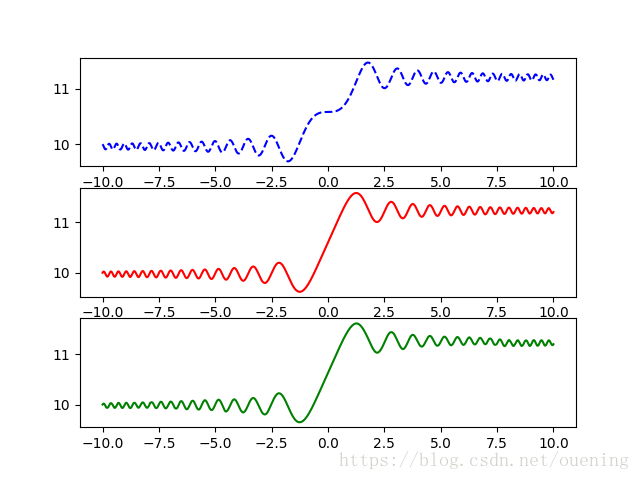
## 1 求解一阶ODE
def f1(y,t):
'''
dy/dt = func(y, t, ...)
'''
return sin(t**2)
def f2(t,y):
'''
在scipy1.1.0版本中odeint引进tfirst参数,其值为True时,func的参数顺序为 t,y
'''
return cos(t**2)
def solve_first_order_ode():
'''
求解一阶ODE
'''
t1 = linspace(-10,10,1000)
y0 = [10] # 为了兼容solve_ivp函数,这里初值要array类型
y1 = odeint(f1,y0,t1)
y2 = odeint(f2,y0,t1,tfirst=True) # 使用tfirst参数
y3 = solve_ivp(f2,(-10.0,10.0), y0, method='LSODA', t_eval=t1) # 注意参数t_span和t_eval的赋值
plt.subplot(311)
plt.plot(t1,y1,'b--')
plt.subplot(312)
plt.plot(t1,y2,'r-')
plt.subplot(313)
plt.plot(y3.t,y3.y[0],'g')
plt.show()
solve_first_order_ode()
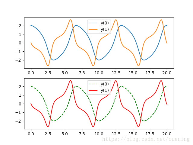
## 2 求解二阶ODE
'''
为了兼容solve_ivp的参数形式,下面例子中的微分方程函数定义的参数顺序为(t,y),因此使用
odeint函数时需要使参数tfirst=True
二阶甚至高阶微分方程组都可以变量替换成一阶方程组的形式,再调用相关函数进行求解,
因此编写函数的时候,不同于一阶微分方程,二阶或者高阶微分方程返回的是低阶到高阶组成的方程组,
具体例子如下:
'''
def fvdp1(t,y):
'''
要把y看出一个向量,y = [dy0,dy1,dy2,...]分别表示y的n阶导,那么
y[0]就是需要求解的函数,y[1]表示一阶导,y[2]表示二阶导,以此类推
'''
dy1 = y[1] # y[1]=dy/dt,一阶导
dy2 = (1 - y[0]**2) * y[1] - y[0] # y[0]是最初始,也就是需要求解的函数
# 注意返回的顺序是[一阶导, 二阶导],这就形成了一阶微分方程组
return [dy1,dy2]
# 或者下面写法更加简单
def fvdp2(t,y):
'''
要把y看出一个向量,y = [dy0,dy1,dy2,...]分别表示y的n阶导
对于二阶微分方程,肯定是由0阶和1阶函数组合而成的,所以下面把y
看成向量的话,y0表示最初始的函数,也就是我们要求解的函数,y1表示
一阶导,对于高阶微分方程也可以以此类推
'''
y0, y1 = y # y0是需要求解的函数,y1是一阶导
# 注意返回的顺序是[一阶导, 二阶导],这就形成了一阶微分方程组
dydt = [y1, (1-y0**2)*y1-y0]
return dydt
def solve_second_order_ode():
'''
求解二阶ODE
'''
t2 = linspace(0,20,1000)
tspan = (0.0, 20.0)
y0 = [2.0, 0.0] # 初值条件
# 初值[2,0]表示y(0)=2,y'(0)=0
# 返回y,其中y[:,0]是y[0]的值,就是最终解,y[:,1]是y'(x)的值
y = odeint(fvdp1, y0, t2, tfirst=True)
y_ = solve_ivp(fvdp2, t_span=tspan, y0=y0, t_eval=t2)
plt.subplot(211)
l1, = plt.plot(t2,y[:,0],label='y(0)')
l2, = plt.plot(t2,y[:,1],label='y(1)')
plt.legend(handles=[l1,l2])
plt.subplot(212)
l3, = plt.plot(y_.t, y_.y[0,:],'g--',label='y(0)')
l4, = plt.plot(y_.t, y_.y[1,:],'r-',label='y(1)')
plt.legend(handles=[l3,l4])
plt.show()
# solve_second_order_ode()
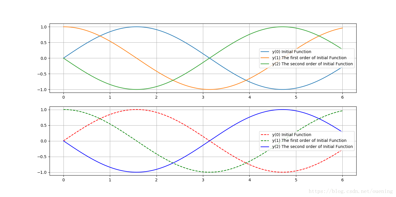
## 3 求解高阶ODE
'''
和前面二阶微分方程一样,只要转换为一阶微分方程组就可以了
'''
def f(t,y):
dy1 = y[1]
dy2 = y[2]
dy3 = -np.cos(t)
return [dy1,dy2,dy3]
def solve_high_order_ode():
'''
求解高阶ODE
'''
t = np.linspace(0,6,1000)
tspan = (0.0, 6.0)
y0 = [0.0, pi, 0.0]
# 初值[0,1,0]表示y(0)=0,y’(0)=1,y''(0)=0
# 返回y, 其中y[:,0]是y[0]的值 ,就是最终解 ,y[:,1]是y’(x)的值
y = odeint(f, y0, t, tfirst=True)
y_ = solve_ivp(f,t_span=tspan, y0=y0, t_eval=t)
plt.subplot(211)
l1, = plt.plot(t,y[:,0],label='y(0) Initial Function')
l2, = plt.plot(t,y[:,1],label='y(1) The first order of Initial Function')
l3, = plt.plot(t,y[:,2],label='y(2) The second order of Initial Function')
plt.legend(handles=[l1,l2,l3])
plt.grid('on')
plt.subplot(212)
l4, = plt.plot(y_.t, y_.y[0,:],'r--', label='y(0) Initial Function')
l5,= plt.plot(y_.t,y_.y[1,:],'g--', label='y(1) The first order of Initial Function')
l6, = plt.plot(y_.t,y_.y[2,:],'b-', label='y(2) The second order of Initial Function')
plt.legend(handles=[l4,l5,l6]) # 显示图例
plt.grid('on')
plt.show()
# solve_high_order_ode()结果分别如下: