代码来源于:tensorflow机器学习实战指南(曾益强 译,2017年9月)——第七章:自然语言处理
代码地址:https://github.com/nfmcclure/tensorflow-cookbook
解决问题:使用“tfidf”来进行垃圾短信的预测(使用逻辑回归算法)
缺点:未考虑单词顺序
TF-IDF:TF词频(Term Frequency),IDF逆向文件频率(Inverse Document Frequency)。
TF表示词条在文档d中出现的频率。
IDF的主要思想是:如果包含词条t的文档越少,也就是分母越小,IDF越大,则说明词条t具有很好的类别区分能力。
i词在j文档中的tfidf值计算
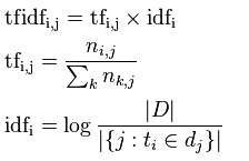
|D|是全部文档数目
分母为有i词的文档数目,有时分母会为0,采用拉普拉斯平滑,作+1处理
步骤如下:
step1:导入需要的包
step2:准备数据集
step3:分词且构建文本向量
step4:分割数据集
step5:构建图
step6:训练效果变化
step1:导入需要的包
import tensorflow as tf
import matplotlib.pyplot as plt
import csv
import numpy as np
import os
import string
import requests
import io
import nltk
from zipfile import ZipFile
from sklearn.feature_extraction.text import TfidfVectorizer
from tensorflow.python.framework import ops
ops.reset_default_graph()

# Start a graph session
sess = tf.Session()

#定义批处理大小和特征向量长度
batch_size = 200
max_features = 1000
step2:准备数据集
step3:分词且构建文本向量
# Define tokenizer
def tokenizer(text):
    words = nltk.word_tokenize(text)
    return words

# Create TF-IDF of texts
tfidf = TfidfVectorizer(tokenizer=tokenizer, stop_words='english', max_features=max_features)
sparse_tfidf_texts = tfidf.fit_transform(texts)
此时sparse_tfidf_texts已经将每个文本转成一个1000维的向量,多个文本构成矩阵(注意该矩阵为稀疏矩阵,查看值使用sparse_tfidf_texts.todense())
step4:分割数据集
# Split up data set into train/test
train_indices = np.random.choice(sparse_tfidf_texts.shape[0], round(0.8*sparse_tfidf_texts.shape[0]), replace=False)
test_indices = np.array(list(set(range(sparse_tfidf_texts.shape[0])) - set(train_indices)))
texts_train = sparse_tfidf_texts[train_indices]
texts_test = sparse_tfidf_texts[test_indices]
target_train = np.array([x for ix, x in enumerate(target) if ix in train_indices])
target_test = np.array([x for ix, x in enumerate(target) if ix in test_indices])
step5:构建图
# Create variables for logistic regression设置权重和偏置项
A = tf.Variable(tf.random_normal(shape=[max_features,1]))
b = tf.Variable(tf.random_normal(shape=[1,1]))

# Initialize placeholders设置数据的占位符
x_data = tf.placeholder(shape=[None, max_features], dtype=tf.float32)
y_target = tf.placeholder(shape=[None, 1], dtype=tf.float32)

# Declare logistic model (sigmoid in loss function)
model_output = tf.add(tf.matmul(x_data, A), b)

# Declare loss function (Cross Entropy loss)损失函数计算
loss = tf.reduce_mean(tf.nn.sigmoid_cross_entropy_with_logits(model_output, y_target))

# Actual Prediction 预测结果
prediction = tf.round(tf.sigmoid(model_output))
predictions_correct = tf.cast(tf.equal(prediction, y_target), tf.float32)
accuracy = tf.reduce_mean(predictions_correct)

# Declare optimizer 用GD优化算法更新权重,最小化损失
my_opt = tf.train.GradientDescentOptimizer(0.0025)
train_step = my_opt.minimize(loss)
step6:训练效果变化
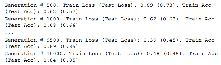
# Intitialize Variables
init = tf.initialize_all_variables()
sess.run(init)

# Start Logistic Regression
train_loss = []
test_loss = []
train_acc = []
test_acc = []
i_data = []
for i in range(10000):
    rand_index = np.random.choice(texts_train.shape[0], size=batch_size)
    rand_x = texts_train[rand_index].todense()
    rand_y = np.transpose([target_train[rand_index]])
    sess.run(train_step, feed_dict={x_data: rand_x, y_target: rand_y})

    # Only record loss and accuracy every 100 generations,100回记录,500回输出状态
    if (i+1)%100==0:
        i_data.append(i+1)
        train_loss_temp = sess.run(loss, feed_dict={x_data: rand_x, y_target: rand_y})
        train_loss.append(train_loss_temp)

        test_loss_temp = sess.run(loss, feed_dict={x_data: texts_test.todense(), y_target: np.transpose([target_test])})
        test_loss.append(test_loss_temp)

        train_acc_temp = sess.run(accuracy, feed_dict={x_data: rand_x, y_target: rand_y})
        train_acc.append(train_acc_temp)

        test_acc_temp = sess.run(accuracy, feed_dict={x_data: texts_test.todense(), y_target: np.transpose([target_test])})
        test_acc.append(test_acc_temp)
    if (i+1)%500==0:
        acc_and_loss = [i+1, train_loss_temp, test_loss_temp, train_acc_temp, test_acc_temp]
        acc_and_loss = [np.round(x,2) for x in acc_and_loss]
        print('Generation # {}. Train Loss (Test Loss): {:.2f} ({:.2f}). Train Acc (Test Acc): {:.2f} ({:.2f})'.format(*acc_and_loss))
结果如下:
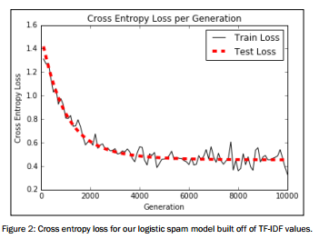
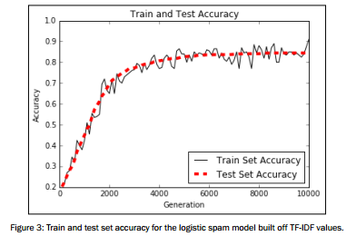
图像展示
# Plot loss over time
plt.plot(i_data, train_loss, 'k-', label='Train Loss')
plt.plot(i_data, test_loss, 'r--', label='Test Loss', linewidth=4)
plt.title('Cross Entropy Loss per Generation')
plt.xlabel('Generation')
plt.ylabel('Cross Entropy Loss')
plt.legend(loc='upper right')
plt.show()

# Plot train and test accuracy
plt.plot(i_data, train_acc, 'k-', label='Train Set Accuracy')
plt.plot(i_data, test_acc, 'r--', label='Test Set Accuracy', linewidth=4)
plt.title('Train and Test Accuracy')
plt.xlabel('Generation')
plt.ylabel('Accuracy')
plt.legend(loc='lower right')
plt.show()