demo演示
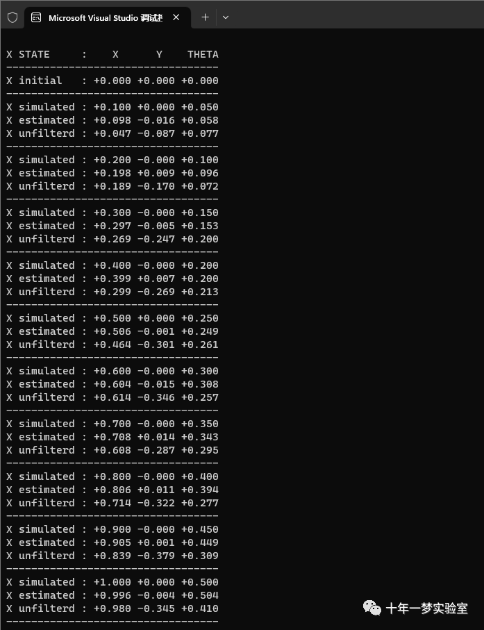
运行结果
我们考虑一个机器人在平面上被少量的准时地标或_信标 包围。
机器人以轴向速度和角速度的形式接收控制动作,并且能够测量信标相对于其自身参考系的位置。
机器人位姿 X 在 SE(2) 中,信标位置 b_k 在 R^2 中,
| cos th -sin th x |
* X = | sin th cos th y | //位置和方向
| 0 0 1 |
* b_k = (bx_k, by_k) // 世界坐标系中的lmk坐标
控制信号 u 是 se(2) 中的旋量,包括纵向速度 v 和角速度 w,没有横向速度分量,在采样时间 dt 上积分。
* u = (v*dt, 0, w*dt)
控制被带有协方差的加性高斯噪声 u_noise 破坏
* Q = diagonal(sigma_v^2, sigma_s^2, sigma_w^2).
此噪声解释了通过 sigma_s 非零值可能出现的横向滑移 u_s,
*当控制 u 到达时,机器人位姿更新为 X <-- X * Exp(u) = X + u。
地标测量是范围和方位类型,但为了简单起见,它们采用笛卡尔形式。
它们的噪声 n 是零均值高斯分布,并用协方差矩阵 R 指定。
我们注意到刚性运动动作 y = h(X,b) = X^-1 * b
* y_k = (brx_k, bry_k) // 机器人坐标系中的lmk坐标
我们考虑位于已知位置的信标 b_k。
我们将要估计的位姿定义为 SE(2) 中的 X。
估计误差 dx 及其协方差 P 在 X 处的切线空间中表示。
*所有这些变量再次总结如下
* * X : 机器人位姿,SE(2)
* u :机器人控制量,(v*dt ; 0 ; w*dt) in se(2)
* Q : 控制扰动协方差
* b_k : 第 k 个地标位置,R^2
* y :机器人坐标系中的笛卡尔地标测量,R^2
* R : 测量噪声的协方差
* The motion and measurement models are运动和测量模型是
* X_(t+1) = f(X_t, u) = X_t * Exp ( w ) //运动方程
* y_k = h(X, b_k) = X^-1 * b_k //测量方程
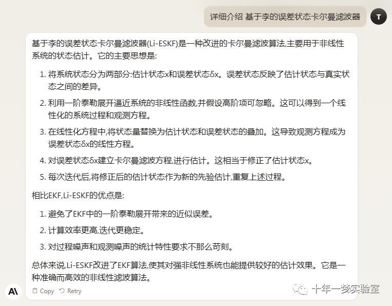
下面的算法首先包括一个模拟器来产生测量结果,然后使用这些测量结果来估计状态,使用基于李的误差状态卡尔曼滤波器。最后,打印模拟状态和估计状态以及未过滤状态(即没有卡尔曼校正)可以评估估计的质量。
#include "manif/SE2.h"


#include <vector>


#include <iostream>
#include <iomanip>


using std::cout;
using std::endl;


using namespace Eigen;


typedef Array<double, 2, 1> Array2d;
typedef Array<double, 3, 1> Array3d;


int main()
{
    std::srand((unsigned int) time(0));


    // START CONFIGURATION
    //
    //
    const int NUMBER_OF_LMKS_TO_MEASURE = 3;


    // Define the robot pose element and its covariance
    manif::SE2d X, X_simulation, X_unfiltered;
    Matrix3d    P;


    X_simulation.setIdentity();
    X.setIdentity();
    X_unfiltered.setIdentity();
    P.setZero();


    // Define a control vector and its noise and covariance
    manif::SE2Tangentd  u_simu, u_est, u_unfilt;
    Vector3d            u_nom, u_noisy, u_noise;
    Array3d             u_sigmas;
    Matrix3d            U;


    u_nom    << 0.1, 0.0, 0.05;
    u_sigmas << 0.1, 0.1, 0.1;
    U        = (u_sigmas * u_sigmas).matrix().asDiagonal();


    // Declare the Jacobians of the motion wrt robot and control
    manif::SE2d::Jacobian J_x, J_u;


    // Define three landmarks in R^2
    Eigen::Vector2d b0, b1, b2, b;
    b0 << 2.0,  0.0;
    b1 << 2.0,  1.0;
    b2 << 2.0, -1.0;
    std::vector<Eigen::Vector2d> landmarks;
    landmarks.push_back(b0);
    landmarks.push_back(b1);
    landmarks.push_back(b2);


    // Define the beacon's measurements
    Vector2d                y, y_noise;
    Array2d                 y_sigmas;
    Matrix2d                R;
    std::vector<Vector2d>   measurements(landmarks.size());


    y_sigmas << 0.01, 0.01;
    R        = (y_sigmas * y_sigmas).matrix().asDiagonal();


    // Declare the Jacobian of the measurements wrt the robot pose
    Matrix<double, 2, 3>    H;      // H = J_e_x


    // Declare some temporaries
    Vector2d                e, z;   // expectation, innovation
    Matrix2d                E, Z;   // covariances of the above
    Matrix<double, 3, 2>    K;      // Kalman gain
    manif::SE2Tangentd      dx;     // optimal update step, or error-state
    manif::SE2d::Jacobian   J_xi_x; // Jacobian is typedef Matrix
    Matrix<double, 2, 3>    J_e_xi; // Jacobian


    //
    //
    // CONFIGURATION DONE


    // DEBUG
    cout << std::fixed   << std::setprecision(3) << std::showpos << endl;
    cout << "X STATE     :    X      Y    THETA" << endl;
    cout << "----------------------------------" << endl;
    cout << "X initial   : " << X_simulation.log().coeffs().transpose() << endl;
    cout << "----------------------------------" << endl;
    // END DEBUG


    // START TEMPORAL LOOP
    //
    //


    // Make 10 steps. Measure up to three landmarks each time.
    for (int t = 0; t < 10; t++)
    {
         I. Simulation ###############################################################################


        /// simulate noise
        u_noise = u_sigmas * Array3d::Random();             // control noise
        u_noisy = u_nom + u_noise;                          // noisy control


        u_simu   = u_nom;
        u_est    = u_noisy;
        u_unfilt = u_noisy;


        /// first we move - - - - - - - - - - - - - - - - - - - - - - - - - - - -
        X_simulation = X_simulation + u_simu;               // overloaded X.rplus(u) = X * exp(u)


        /// then we measure all landmarks - - - - - - - - - - - - - - - - - - - -
        for (std::size_t i = 0; i < landmarks.size(); i++)
        {
            b = landmarks[i];                               // lmk coordinates in world frame


            /// simulate noise
            y_noise = y_sigmas * Array2d::Random();         // measurement noise


            y = X_simulation.inverse().act(b);              // landmark measurement, before adding noise
            y = y + y_noise;                                // landmark measurement, noisy
            measurements[i] = y;                            // store for the estimator just below
        }


         II. Estimation ###############################################################################


        /// First we move - - - - - - - - - - - - - - - - - - - - - - - - - - - -


        X = X.plus(u_est, J_x, J_u);                        // X * exp(u), with Jacobians


        P = J_x * P * J_x.transpose() + J_u * U * J_u.transpose();


        /// Then we correct using the measurements of each lmk - - - - - - - - -
        for (int i = 0; i < NUMBER_OF_LMKS_TO_MEASURE; i++)
        {
            // landmark
            b = landmarks[i];                               // lmk coordinates in world frame


           // measurement
            y = measurements[i];                            // lmk measurement, noisy


            // expectation
            e = X.inverse(J_xi_x).act(b, J_e_xi);           // note: e = R.tr * ( b - t ), for X = (R,t).
            H = J_e_xi * J_xi_x;                            // note: H = J_e_x = J_e_xi * J_xi_x
            E = H * P * H.transpose();


            // innovation
            z = y - e;
            Z = E + R;


            // Kalman gain
            K = P * H.transpose() * Z.inverse();            // K = P * H.tr * ( H * P * H.tr + R).inv


            // Correction step
            dx = K * z;                                     // dx is in the tangent space at X


            // Update
            X = X + dx;                                     // overloaded X.rplus(dx) = X * exp(dx)
            P = P - K * Z * K.transpose();
        }


         III. Unfiltered ##############################################################################


        // move also an unfiltered version for comparison purposes
        X_unfiltered = X_unfiltered + u_unfilt;


         IV. Results ##############################################################################


        // DEBUG
        cout << "X simulated : " << X_simulation.log().coeffs().transpose() << endl;
        cout << "X estimated : " << X.log().coeffs().transpose() << endl;
        cout << "X unfilterd : " << X_unfiltered.log().coeffs().transpose() << endl;
        cout << "----------------------------------" << endl;
        // END DEBUG


    }


    //
    //
    // END OF TEMPORAL LOOP. DONE.


    return 0;
}
The End