1 原理简介
微分方程可以写成2部分:
- 第一部分满足初始和边界条件并包含不可调节参数
- 第二部分不会影响第一部分,这部分涉及前馈神经网络,包含可调节参数(权重)。
因此在构建微分方程的函数时,要满足上述两个条件,今天就来简单看下。
假设存在以下微分方程:

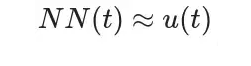
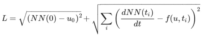
上述微分方程f对应着一个函数u(t),同时满足初始条件u(0)=u_0,为此可以令:
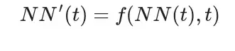
则NN(t)的导数为:
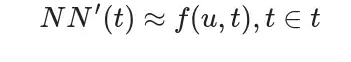
根据以上等式,NN(t)的导数近似于:
可以把上式转换成损失函数:
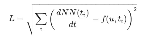
简而言之,就是已知微分函数,然后用神经网络去拟合该微分函数的原函数,然后用微分公式作为损失函数去逼近原微分函数。
微分公式:

此外,还需要将初始条件考虑进去:
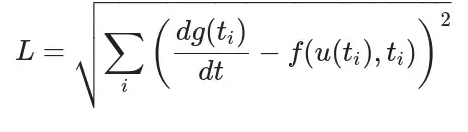
上述并不是一个好的方法,损失项越多会影响稳定性。为此会定义一个新函数,该函数要满足初始条件同时是t的函数:

则损失函数为:
注意,神经微分网络目前主要是去近似一些简单的微分函数,复杂的比较消耗时间以及需要高算力。
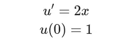
2 实践
假设存在下述微分函数和网络:
import tensorflow as tf
import matplotlib.pyplot as plt
import numpy as np
np.random.seed(123)
tf.random.set_seed(123)
"""微分初始条件以及相应参数定义"""
f0 = 1 # 初始条件 u(0)=1
# 用于神经网络求导,无限小的小数
inf_s = np.sqrt(np.finfo(np.float32).eps)
learning_rate = 0.01
training_steps = 500
batch_size = 100
display_step = training_steps/10
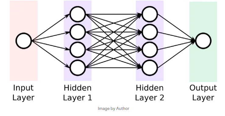
"""神经网络参数定义"""
n_input = 1 # 输入维度
n_hidden_1 = 32 # 第一层输出维度
n_hidden_2 = 32 # 第二层输出维度
n_output = 1 # 最后一层输出维度
weights = {
'h1': tf.Variable(tf.random.normal([n_input, n_hidden_1])),
'h2': tf.Variable(tf.random.normal([n_hidden_1, n_hidden_2])),
'out': tf.Variable(tf.random.normal([n_hidden_2, n_output]))
}
biases = {
'b1': tf.Variable(tf.random.normal([n_hidden_1])),
'b2': tf.Variable(tf.random.normal([n_hidden_2])),
'out': tf.Variable(tf.random.normal([n_output]))
}
"""优化器"""
optimizer = tf.optimizers.SGD(learning_rate)
"""定义模型和损失函数"""
"""多层感知机"""
def multilayer_perceptron(x):
x = np.array([[[x]]], dtype='float32')
layer_1 = tf.add(tf.matmul(x, weights['h1']), biases['b1'])
layer_1 = tf.nn.sigmoid(layer_1)
layer_2 = tf.add(tf.matmul(layer_1, weights['h2']), biases['b2'])
layer_2 = tf.nn.sigmoid(layer_2)
output = tf.matmul(layer_2, weights['out']) + biases['out']
return output
"""近似原函数"""
def g(x):
return x * multilayer_perceptron(x) + f0
"""微分函数"""
def f(x):
return 2*x
"""定义损失函数逼近导数"""
def custom_loss():
summation = []
# 注意这里,没有定义数据,根据函数中t的范围选取了10个点进行计算
for x in np.linspace(0,1,10):
dNN = (g(x+inf_s)-g(x))/inf_s
summation.append((dNN - f(x))**2)
return tf.reduce_mean(tf.abs(summation))
"""训练函数"""
def train_step():
with tf.GradientTape() as tape:
loss = custom_loss()
trainable_variables=list(weights.values())+list(biases.values())
gradients = tape.gradient(loss, trainable_variables)
optimizer.apply_gradients(zip(gradients, trainable_variables))
"""训练模型"""
for i in range(training_steps):
train_step()
if i % display_step == 0:
print("loss: %f " % (custom_loss()))
"""绘图"""
from matplotlib.pyplot import figure
figure(figsize=(10,10))
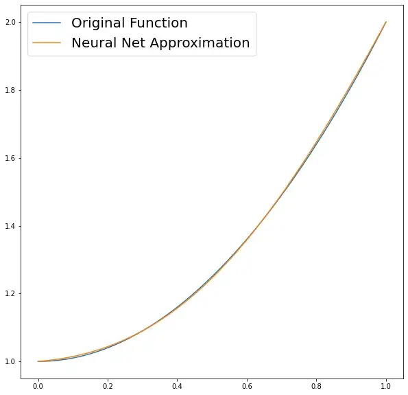
# True Solution (found analitically)
def true_solution(x):
return x**2 + 1
X = np.linspace(0, 1, 100)
result = []
for i in X:
result.append(g(i).numpy()[0][0][0])
S = true_solution(X)
plt.plot(X, S, label="Original Function")
plt.plot(X, result, label="Neural Net Approximation")
plt.legend(loc=2, prop={
'size': 20})
plt.show()
参考:
https://towardsdatascience.com/using-neural-networks-to-solve-ordinary-differential-equations-a7806de99cdd