Python Matplotlib习题

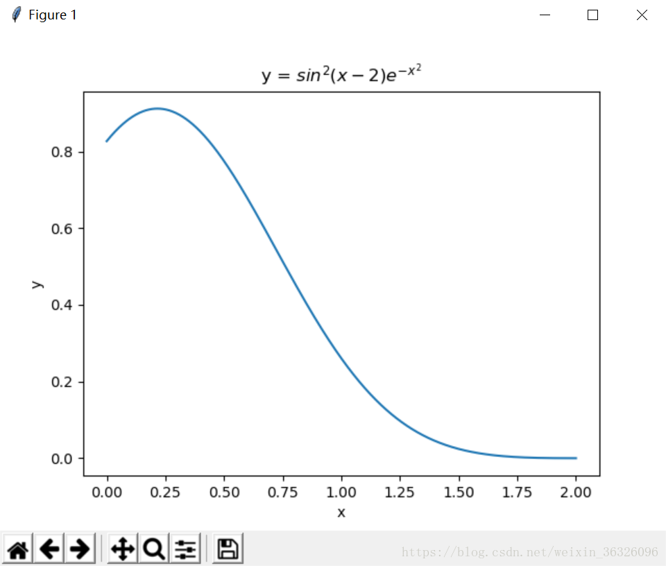
Exercise 11.1: Plotting a function

Plot the function $f(x) = sin^2(x-2){e^{-x^2}}$ over the interval [0, 2]. Add proper axis labels, a title, etc.

代码：

import numpy as np
import matplotlib.pyplot as plt
import math

x = np.linspace(0, 2, 1000) 
y = [math.sin(i-2)**2 * math.exp(-i**2) for i in x]  
plt.plot(x, y)  
plt.xlabel('x')
plt.ylabel('y')
plt.title('y = $sin^2(x-2){e^{-x^2}}$')
plt.show()

运行效果：

Exercise 11.2: Data

Create a data matrix $X$ with 20 observations of 10 variables. Generate a vector $b$ with parameters Then generate the response vector $y = Xb+z$ where $z$ is a vector with standard normally distributed variables.
Now (by only using $y$ and $X$), find an estimator for $b$, by solving $\hat{b} = \arg \min \limits_{b} ||Xb - y||_2$. Plot the true parameters $b$ and estimated parameters $\hat{b}$. See Figure 1 for an example plot.

一开始这题我是不会的，后来看到网上的资料说这道题可以用scipy.optimize库中的minimize函数。minimize函数进行的是多变量的最小化，原型为scipy.optimize.minimize(fun, x0, args=(), method=None, jac=None, hess=None, hessp=None, bounds=None, constraints=(), tol=None, callback=None, options=None)，fun是需要进行最小化的函数，x0是初步猜测，这里一开始猜测为0向量，arg是额外参数。

代码：

import numpy as np    
import matplotlib.pyplot as plt  
import scipy as sp   
from scipy.optimize import minimize   

def error(b0, X, y):  
    b0 = np.reshape(b0, (10, 1))  
    return np.linalg.norm(np.dot(X, b0) - y)  

n = 20
m = 10  
X = np.random.randint(1, 4, (n, m))  
X = np.mat(X)  
b = np.random.randint(-2, 2,(1, m))  
b_vec = (np.mat(b)).T  
z = np.random.randn(1, n)  
z_vec = (np.mat(z)).T  
y_vec = np.dot(X, b_vec) + z_vec  
y = np.array(y_vec)  
b0 = np.zeros((10, 1))  
Para = minimize(error, b0, args=(X, y))  
b_ = Para.x    
x1 = np.linspace(0, 9, 10)  
fig = plt.figure()
p1 = plt.scatter(x1, b, marker='x', color='r')  
p2 = plt.scatter(x1, b_, marker='o', color='b')  
plt.xlim(0, 10)  
plt.ylim(-3, 3)  
plt.xlabel('index')  
plt.ylabel('value')  
plt.legend([p1, p2], ['True coefficents', 'Estimated coefficients'])  
plt.show()

运行效果：

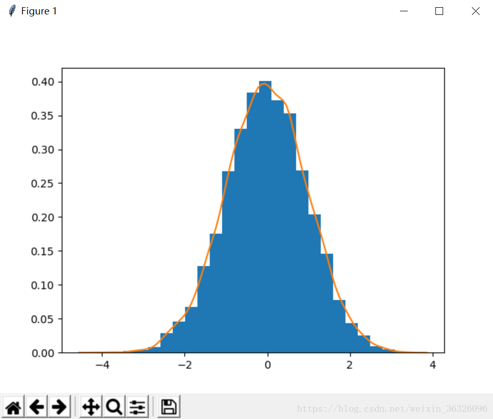
Exercise 11.3: Histogram and density estimation

Generate a vector $z$ of 10000 observations from your favorite exotic distribution. Then make a plot that shows a histogram of $z$ (with 25 bins), along with an estimate for the density, using a Gaussian kernel density estimator (see scipy.stats). See Figure 2 for an example plot.

代码：

import numpy as np  
import matplotlib.pyplot as plt  
import seaborn  

x = np.random.randn(10000)
plt.hist(x, 25, normed=1)  
seaborn.kdeplot(x)  
plt.show()

运行效果：