Exercise 11.1: Plotting a function Plot thefunction
f(x) = sin2(x−2)e−x2 over the interval [0,2]. Add proper axis labels, a title, etc.
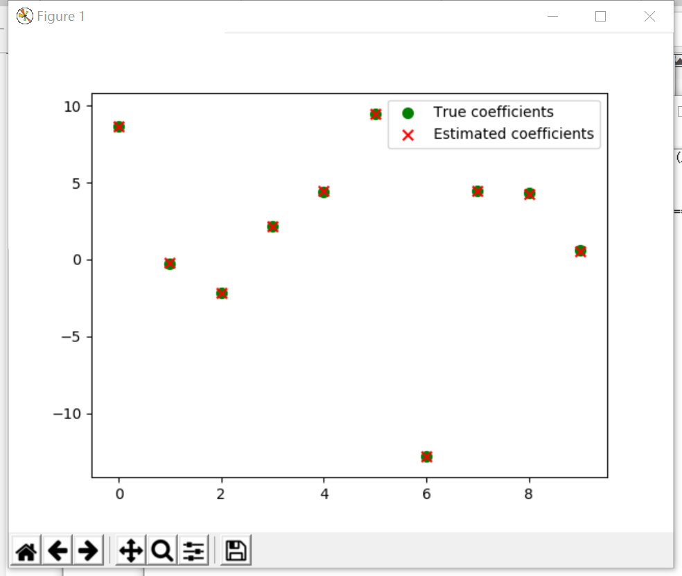
Exercise 11.2: Data Create a data matrix Xwith 20 observations of 10 variables. Generate a vector b with parameters Thengenerate the response vector y = Xb+z where z is a vector with standardnormally distributed variables.
Now (by only using y and X), find an estimator for b, by solving
ˆ b = argmin b kXb−yk2
Plot the true parameters b and estimatedparameters ˆ b. See Figure 1 for an example plot.
Exercise 11.3: Histogram and densityestimation Generate a vector z of 10000 observations from your favorite exoticdistribution. Then make a plot that shows a histogram of z (with 25 bins),along with an estimate for the density, using a Gaussian kernel densityestimator (see scipy.stats). See Figure 2 for an example plot.
ex 11.1
import matplotlib.pyplot as plt
import numpy as np

x = np.linspace(0, 2, 50)
y = (np.sin(x-2)**2) * (np.e**(-x**2))
plt.plot(x, y)
plt.show()

ex 11.2
import matplotlib.pyplot as plt
import numpy
import random
import scipy.stats as stats
import numpy.linalg


X = numpy.random.randn(20, 10) * random.randint(1, 10)
b = numpy.random.randn(10, 1) * random.randint(1, 10)
z = numpy.random.randn(20, 1)
Y = numpy.dot(X, b) + z
b_ = numpy.linalg.lstsq(X, Y, rcond=None)[0]
print(b)
print(b_)
plt.scatter(range(10), list(b.T), s=50, marker='o', c='g')
plt.scatter(range(10), list(b_.T), s=50, marker='x', c='r')
plt.legend(['True coefficients','Estimated coefficients'])
plt.show()
ex 11.3
import numpy as np
import matplotlib.pyplot as plt
import seaborn

x = np.random.randn(10000)
plt.hist(x, 25, normed=1)
seaborn.kdeplot(x)
plt.show()

2018/5/29