梯度下降算法实战

梯度下降算法实战

上篇我们详细解释了梯度下降算法的数学原理，查看上篇数学原理请点击这里，本篇主要实战梯度下降算法，用一个简单的线性回归来展示梯度下降算法迷人的魅力。不懂原理党的同学也可以直接撸代码，碰到问题后再逐一查找资料，如果往更高层次的方向发展，那么数学肯定是必不可少的，必定要回归到最基础的地方。好了！废话不多说，直接上代码！

1、资料来源

资料为自己编的，当然你可以自行收集资料或者下载资料，资料如下

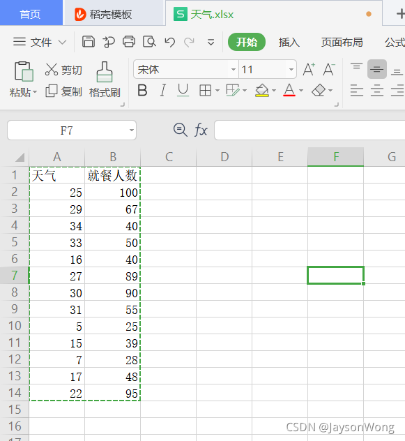
天气	就餐人数
25	100
29	67
34	40
33	50
16	40
27	89
30	90
31	55
5	25
15	39
7	28
17	48
22	95

资料为xlsx格式，保存在D盘根目录，资料图如下：

2、代码

# -*- coding: utf-8 -*-
"""
AUTHOR: jsonwong
TIME: 2021/9/17
"""

import pandas as pd
import numpy as np
import matplotlib.pyplot as plt

def data_process(file_path): # 数据处理函数
    data = pd.read_excel(file_path, header=None, names=['weather', 'number'])
    new_data = data.drop([0])
    new_data.insert(0, 'Ones', 1)
    return new_data

def vectorization(data): # 向量化函数
    cols = data.shape[1]
    X = data.iloc[:, 0:cols-1]  # 取前cols-1列，即输入向量
    y = data.iloc[:, cols-1:cols]  # 取最后一列，即目标向量
    X = np.matrix(X.values)
    y = np.matrix(y.values)
    return X, y

def ComputerCost(X, y, theta): # cost function代价函数
    inner = np.power(((X * theta.T) - y), 2)
    return np.sum(inner) / (2 * len(X))

def gradientDescent(X, y, theta, alpha, epoch): # 梯度下降函数
    temp = np.matrix(np.zeros(theta.shape))  # 初始化一个 θ 临时矩阵(1, 2)
    parameters = int(theta.flatten().shape[1])  # 参数 θ的数量
    cost = np.zeros(epoch)  # 初始化一个ndarray，包含每次epoch的cost
    m = X.shape[0]  # 样本数量m

    for i in range(epoch):
        # 利用向量化一步求解
        temp = theta - (alpha / m) * (X * theta.T - y).T * X
        theta = temp
        cost[i] = ComputerCost(X, y, theta)
    return theta, cost

def visualization(new_data, final_theta, *cost): # 可视化函数
    x = new_data["weather"].values # 横坐标
    # x = np.linspace(new_data.weather.min(), new_data.weather.max(), 6)  # 横坐标
    f = final_theta[0, 0] + (final_theta[0, 1] * x)  # 纵坐标
    plt.plot(x, f, 'r', label='Prediction')
    plt.scatter(new_data.weather, new_data.number, label='Traning Data')
    plt.legend(loc=2)  # 2表示在左上角
    plt.xlabel('weather')
    plt.ylabel('number')
    plt.title('Predicted')
    plt.savefig('D:/predicted')
    plt.show()

def iteration_figure(epoch, cost): # 迭代图像函数
    plt.plot(np.arange(epoch), cost, 'r')
    plt.xlabel('epoch')
    plt.ylabel('cost')
    plt.title('error with epoch')
    plt.savefig('D:/error figure')
    plt.show()

def main():
    file_path = 'D:/天气.xlsx'
    theta = np.matrix([0, 0]) # 初始化theta
    new_data = data_process(file_path)
    X, y = vectorization(new_data)
    final_theta, cost = gradientDescent(X, y, theta, 0.003, 10000)
    visualization(new_data, final_theta)
    iteration_figure(10000, cost)

if __name__ == '__main__':
    main()

3、结果

线性回归结果如下图：

可以用EXCEL画同样的拟合直线，如下图，可以看到与我们拟合的图像几乎一致（不一致，需要调整迭代次数与学习率α）

拟合过程如下图：