梯度下降优化算法

1. Gradient descent

Gradient descent is a way to minimize an objective function $J(\theta)$ parameterized by a model’s parameters $\theta\in\mathbb{R}^d$ by updating the parameters in the opposite direction of the gradient of the objective function $\nabla_\theta J(\theta)$ . The learning rate $\eta$ determines the size of the steps we take to reach a (local) minimum.

2. Gradient descent 3 variants

1. Batch gradient descent

Batch gradient descent computes $\nabla_\theta J(\theta)$ for the entire training dataset $X$ and $y$ every time just to perform one update:

θ = θ - η \cdot \nabla θ J (θ; X; y)

$\theta=\theta-\eta\cdot\nabla_\theta J(\theta;X;y)$

Batch gradient descent can be very slow and intractable for large datasets that don’t fit in memory.
It also doesn’t allow us to update our model online.
It is guaranteed to converge to the global minimum for convex error surfaces and to a local minimum for non-convex surfaces.

2. Stochastic gradient descent

Stochastic gradient descent (SGD) in contrast computes $\nabla_\theta J(\theta)$ for each training example $x^{(i)}$ and $y^{(i)}$ to perform one update:

θ = θ - η \cdot \nabla θ J (θ; x (i); y (i))

$\theta=\theta-\eta\cdot\nabla_\theta J(\theta;x^{(i)};y^{(i)})$

Batch gradient descent performs redundant computations for large datasets, as it recomputes gradients for similar examples before each parameter update. SGD does away with this redundancy by performing one update at a time. It is therefore usually much faster.
It can also be used to learn online.
It performs frequent updates with a high variance that cause the objective function to fluctuate heavily. This fluctuation, on the one hand, enables it to jump to new and potentially better local minima. On the other hand, this ultimately complicates convergence to the exact minimum, as It will keep overshooting. However, when we slowly decrease the learning rate (annealing learning rate), It shows the same convergence behaviour as batch gradient descent.
tricks: shuffle the training data at every epoch.

3. Mini-batch gradient descent

Mini-batch gradient descent finally takes the best of both worlds, i.e. it performs an update for every mini-batch of $n$ training examples $x^{(i:i+n)}$ and $y^{(i:i+n)}$ :

θ = θ - η \cdot \nabla θ J (θ; x (i : i + n); y (i : i + n))

$\theta=\theta-\eta\cdot\nabla_\theta J(\theta;x^{(i:i+n)};y^{(i:i+n)})$

It reduces the variance of the parameter updates, which can lead to more stable convergence.
It can make use of highly optimized matrix optimizations common to state-of-the-art deep learning libraries that make computing the gradient w.r.t. a mini-batch very efficient.
tricks: Common mini-batch sizes range between 50 and 256.

4. Challenges

Choosing a proper learning rate can be difficult. A learning rate that is too small leads to painfully slow convergence, while a learning rate that is too large can hinder convergence and cause the loss function to fluctuate around the minimum or even to diverge.
Learning rate schedules try to adjust the learning rate during training by e.g. annealing, i.e. reducing the learning rate according to a pre-defined schedule or when the change in objective between epochs falls below a threshold. These schedules and thresholds, however, have to be defined in advance and are thus unable to adapt to a dataset’s characteristics.
The same learning rate applies to all parameter updates. If our data is sparse and our features have very different frequencies, we might not want to update all of them to the same extent, but perform a larger update for rarely occurring features.
Avoiding getting trapped in numerous suboptimal local minima. The difficulty arises in fact not from local minima but from saddle points, i.e. points where one dimension slopes up and another slopes down. These saddle points are usually surrounded by a plateau of the same error, which makes it notoriously hard for SGD to escape, as the gradient is close to zero in all dimensions.

3. Gradient descent optimization algorithms

We will outline some algorithms that are widely used by the deep learning community to deal with the aforementioned challenges, but not discuss algorithms that are infeasible to compute in practice for high-dimensional data sets, e.g. second-order methods such as Newton’s method.

1. Momentum

SGD has trouble navigating ravines, i.e. areas where the surface curves much more steeply in one dimension than in another, which are common around local optima. In these scenarios, SGD oscillates across the slopes of the ravine while only making hesitant progress along the bottom towards the local optimum (left).

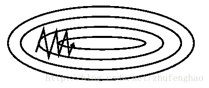
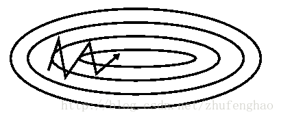
Momentum is a method that helps accelerate SGD in the relevant direction and dampens oscillations (right). It does this by adding a fraction $\gamma$ (set around 0.9) of the update vector of the past time step to the current update vector:

v t θ = = γ v t - 1 - η \nabla θ J (θ) θ + v t

$\begin{array}{rcl} v_t & = & \gamma v_{t-1}-\eta\nabla_\theta J(\theta)\\ \theta & = & \theta+v_t \end{array}$

Theano code:

for p, g in zip(params, grads):
    v = shared(p.get_value() * 0., borrow=True)
    updates.append([p, p + v])
    updates.append([v, momentum * v - lr * g])

The momentum term increases for dimensions whose gradients point in the same directions and reduces updates for dimensions whose gradients change directions. As a result, we gain faster convergence and reduced oscillation.

Another way to use momentum: dampen both velocity and gradient.

v t θ = = γ v t - 1 + (1 - η) \nabla θ J (θ) θ - η v t

$\begin{array}{rcl} v_t & = & \gamma v_{t-1}+(1-\eta)\nabla_\theta J(\theta)\\ \theta & = & \theta-\eta v_t \end{array}$

Theano code:

for p, g in zip(params, grads):
    v = shared(p.get_value() * 0., borrow=True)
    updates.append([v, momentum * v + (1. - momentum) * g])
    updates.append([p, p - lr * v])

2. Nesterov accelerated gradient

Nesterov accelerated gradient (NAG) is a way to give our momentum term more prescience. We know that we will use our momentum term $\gamma v_{t-1}$ to move the parameters $\theta$ . Computing $\theta-\gamma v_{t-1}$ thus gives us an approximation of the next position of the parameters (regardless of the gradient), a rough idea where our parameters are going to be. We can now effectively look ahead by calculating the gradient not w.r.t. to our current parameters $\theta$ but w.r.t. the approximate future position of our parameters (fraction $\gamma$ similiar to momentum):

v t θ t + 1 = = γ v t - 1 - η \nabla θ J (θ t - γ v t - 1) θ t + v t

$\begin{array}{rcl} v_t & = & \gamma v_{t-1}-\eta\nabla_\theta J(\theta_t-\gamma v_{t-1})\\ \theta_{t+1} & = & \theta_t+v_t \end{array}$

with $\theta_t-\gamma v_{t-1}$ repalced by $\hat{\theta}_t$ to obtain

v t θ ̂ t + 1 = = = γ v t - 1 - η \nabla θ J (θ ̂ t) θ ̂ t + γ v t - η \nabla θ J (θ ̂ t) θ ̂ t + γ 2 v t - 1 - (1 + γ) η \nabla θ J (θ ̂ t)

$\begin{array}{rcl} v_t & = & \gamma v_{t-1}-\eta\nabla_\theta J(\hat{\theta}_t)\\ \hat{\theta}_{t+1} & = & \hat{\theta}_t+\gamma v_t-\eta\nabla_\theta J(\hat{\theta}_t)\\ & = & \hat{\theta}_t+\gamma^2 v_{t-1}-(1+\gamma)\eta\nabla_\theta J(\hat{\theta}_t) \end{array}$

Theano code:

for p, g in zip(params, grads):
    v = shared(p.get_value() * 0., borrow=True)
    updates.append([v, momentum * v - lr * g])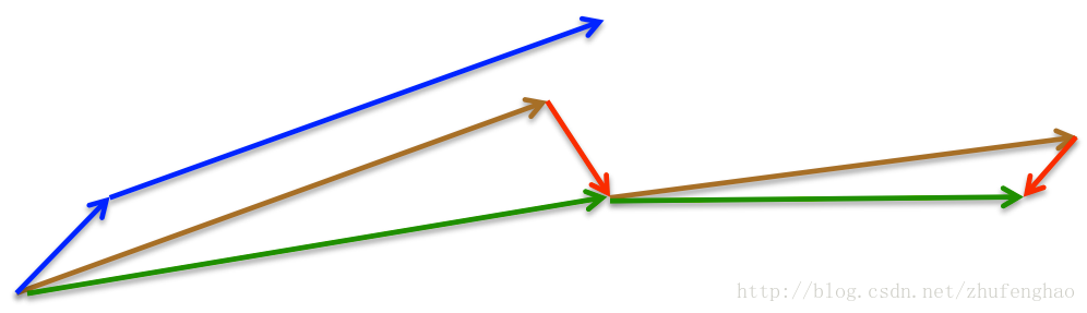
    updates.append([p, p + momentum * v - lr * g])

Momentum first computes the current gradient (small blue vector) and then takes a big jump in the direction of the updated accumulated gradient (big blue vector).
NAG first makes a big jump (brown vector) in the direction of the previous accumulated gradient, measures the gradient and then makes a correction (red vector) and get the updated accumulated gradient (green vector). This anticipatory update prevents us from going too fast and results in increased responsiveness, which has significantly increased the performance of RNNs on a number of tasks.

3. Adagrad

Adagrad is an algorithm for gradient-based optimization that just adapts the learning rate to the parameters, performing larger updates for infrequent and smaller updates for frequent parameters. For this reason, it is well-suited for dealing with sparse data. Adagrad uses a different learning rate for every parameter $\theta_i$ at every time step $t$ , we set $g_{t,i}$ to be the gradient of the objective function w.r.t. to the parameter $\theta_i$ at time step $t$ , Adagrad’s update rule is to modify the general learning rate $\eta$ at each time step $t$ for every parameter $\theta_i$ based on the past gradients that have been computed for $\theta_i$ :

g t, i G t, i i θ t + 1, i = = = \nabla θ J (θ i) \sum τ = 1 t g 2 τ, i θ t, i - η G t , i i + ϵ ‾ ‾ ‾ ‾ ‾ ‾ ‾ ‾ \sqrt \cdot g t, i

$\begin{array}{rcl} g_{t,i}& = &\nabla_\theta J(\theta_i)\\ G_{t,ii}& = &\sum_{\tau=1}^{t}g_{\tau,i}^2\\ \theta_{t+1,i}& = &\theta_{t,i}-\frac{\eta}{\sqrt{G_{t,ii}+\epsilon}}\cdot g_{t,i} \end{array}$

$G_t \in \mathbb{R}^{d\times d}$ is a diagonal matrix where each diagonal element $G_{t,ii}$ is the sum of the squares of the gradients w.r.t. $\theta_i$ up to time step $t$ , while $\epsilon$ is a smoothing term that avoids division by zero (usually on the order of 1e−8). Interestingly, without the square root operation, the algorithm performs much worse.

Theano code:

for p, g in zip(params, grads):
    acc = shared(p.get_value() * 0., borrow=True)
    accNew = acc + T.square(g)
    g = g / T.sqrt(accNew + epsilon)
    updates.append((acc, accNew))
    updates.append((p, p - lr * g))

benefits: eliminate the need to manually tune the learning rate. Just use a default value of 0.01 and leave it at that.
weakness: accumulation of the squared gradients in the denominator keeps growing during training, which causes the learning rate to shrink and eventually become infinitesimally small, at which point the algorithm is no longer able to acquire additional knowledge.

4. Adadelta

Adadelta is an extension of Adagrad that seeks to reduce its aggressive, monotonically decreasing learning rate. Instead of accumulating all past squared gradients, Adadelta restricts the window of accumulated past gradients to some fixed size $w$ . Instead of inefficiently storing $w$ previous squared gradients, the sum of gradients is recursively defined as a decaying average of all past squared gradients. The running average $E[g^2]_t$ at time step $t$ then depends only on the previous average and the current gradient (fraction $\gamma$ similiar to momentum). The parameter update vector of Adadelta thus change the form of adagrad as:

E [g 2] t R M S [g] t Δ θ t = \equiv = γ E [g 2] t - 1 + (1 - γ) g 2 t E [g 2] t + ϵ ‾ ‾ ‾ ‾ ‾ ‾ ‾ ‾ ‾ \sqrt - η R M S [ g ] t g t

$\begin{array}{rcl} E[g^2]_t& = &\gamma E[g^2]_{t-1}+(1-\gamma)g_t^2\\ RMS[g]_t& \equiv &\sqrt{E[g^2]_t+\epsilon}\\ \Delta\theta_t& = &-\frac{\eta}{RMS[g]_t}g_t \end{array}$

To make the units in this update have the same hypothetical units as the parameter, we define another exponentially decaying average, not of squared gradients but of squared parameter updates:

E [Δ θ 2] t R M S [Δ θ] t = \equiv γ E [Δ θ 2] t - 1 + (1 - γ) Δ θ 2 t E [Δ θ 2] t + ϵ ‾ ‾ ‾ ‾ ‾ ‾ ‾ ‾ ‾ ‾ ‾ \sqrt

$\begin{array}{rcl} E[\Delta\theta^2]_t& = &\gamma E[\Delta\theta^2]_{t-1}+(1-\gamma)\Delta\theta_t^2\\ RMS[\Delta\theta]_t& \equiv &\sqrt{E[\Delta\theta^2]_t+\epsilon} \end{array}$

Since $RMS[\Delta\theta]_t$ is unknown, we approximate it with $RMS[\Delta\theta]_{t-1}$ (the RMS of parameter updates until the previous time step). Replacing the learning rate $\eta$ in the previous update rule with $RMS[\Delta\theta]_{t-1}$ finally yields the Adadelta update rule:

Δ θ t θ t + 1 = = - R M S [ Δ θ ] t - 1 R M S [ g ] t g t θ t + Δ θ t

$\begin{array}{rcl} \Delta\theta_t& = &-\frac{RMS[\Delta\theta]_{t-1}}{RMS[g]_t}g_t\\ \theta_{t+1}& = &\theta_t+\Delta\theta_t \end{array}$

Theano code:

for p, g in zip(params, grads):
    acc = shared(p.get_value() * 0., borrow=True)
    accDelta = shared(p.get_value() * 0., borrow=True)
    accNew = rho * acc + (1 - rho) * T.square(g)
    delta = g * T.sqrt(accDelta + epsilon) / T.sqrt(accNew + epsilon)
    accDeltaNew = rho * accDelta + (1 - rho) * T.square(delta)
    updates.append((acc, accNew))
    updates.append((p, p - lr * delta))
    updates.append((accDelta, accDeltaNew))

Note that we do not even need to set a default learning rate, as it has been eliminated from the update rule.

5. RMSprop

RMSprop, like Adadelta, is developed to resolve Adagrad’s radically diminishing learning rates. RMSprop in fact is identical to the first update vector of Adadelta:

E [g 2] t R M S [g] t Δ θ t θ t + 1 = \equiv = = γ E [g 2] t - 1 + (1 - γ) g 2 t E [g 2] t + ϵ ‾ ‾ ‾ ‾ ‾ ‾ ‾ ‾ ‾ \sqrt - η R M S [ g ] t g t θ t + Δ θ t

$\begin{array}{rcl} E[g^2]_t& = &\gamma E[g^2]_{t-1}+(1-\gamma)g_t^2\\ RMS[g]_t& \equiv &\sqrt{E[g^2]_t+\epsilon}\\ \Delta\theta_t& = &-\frac{\eta}{RMS[g]_t}g_t\\ \theta_{t+1}& = &\theta_t+\Delta\theta_t \end{array}$

RMSprop as well divides the learning rate by an exponentially decaying average of squared gradients. Hinton suggests $\gamma$ to be set to 0.9, and the learning rate $\eta$ to default 0.001.

Theano code:

for p, g in zip(params, grads):
    acc= shared(p.get_value() * 0., borrow=True)  # 加权累加器
    accNew = rho * acc + (1 - rho) * T.square(g)
    g = g / T.sqrt(accNew + epsilon)
    updates.append((acc, accNew))
    updates.append((p, p - lr * g))

6. Adam

Adaptive Moment Estimation (Adam) is another method that computes adaptive learning rates for each parameter. It stores not only an exponentially decaying average of past squared gradients $v_t$ (like Adadelta and RMSprop), but also an exponentially decaying average of past gradients $m_t$ (like momentum):

m t v t = = β 1 m t - 1 + (1 - β 1) g t β 2 v t - 1 + (1 - β 2) g 2 t

$\begin{array}{rcl} m_t& = &\beta_1m_{t-1}+(1-\beta_1)g_t\\ v_t& = &\beta_2v_{t-1}+(1-\beta_2)g_t^2\\ \end{array}$

$m_t$ and $v_t$ are estimates of the first moment (the mean) and the second moment (the uncentered variance) of the gradients respectively. But as $m_t$ and $v_t$ are initialized as vectors of 0’s, the authors of Adam observe that they are towards zero with bias, especially during the initial time steps, and especially when the decay rates are small (i.e. $\beta_1$ and $\beta_2$ are close to 1). So they counteract these biases by computing bias-corrected first and second moment estimates (using the power $t$ of $\beta_1$ and $\beta_2$ ):

m ̂ t v ̂ t = = m t 1 - β t 1 v t 1 - β t 2

$\begin{array}{rcl} \hat{m}_t& = &\frac{m_t}{1-\beta_1^t}\\ \hat{v}_t& = &\frac{v_t}{1-\beta_2^t} \end{array}$

They then use these to update the parameters (like Adadelta and RMSprop), which yields the Adam update rule:

θ t + 1 = θ t - η v ̂ t ‾ ‾ \sqrt + ϵ m ̂ t

$\theta_{t+1}=\theta_{t}-\frac{\eta}{\sqrt{\hat{v}_t}+\epsilon}\hat{m}_t$

The authors propose default values of 0.9 for $\beta_1$ , 0.999 for $\beta_2$ , and 1e−8 for $\epsilon$ .

Theano code:

for p, g in zip(params, grads):
    mt = shared(p.get_value() * 0., borrow=True)
    vt = shared(p.get_value() * 0., borrow=True)
    mtNew = (beta1 * mt) + (1\. - beta1) * g
    vtNew = (beta2 * vt) + (1\. - beta2) * T.square(g)
    pNew = p - lr * mtNew / (T.sqrt(vtNew) + epsilon)
    updates.append((mt, mtNew))
    updates.append((vt, vtNew))
    updates.append((p, pNew))

4. Chosing optimizer

If input data is sparse, using one of the adaptive learning-rate methods
RMSprop $\approx$ Adadelta $\le$ Adam

5. strategies for optimizing gradient descent

1. Parallelizing and distributing SGD to speed up

SGD by itself is inherently sequential: Step-by-step, we progress further towards the minimum. Running SGD can be slow particularly on large datasets. In contrast, running it asynchronously is faster, but suboptimal communication between workers can lead to poor convergence. Additionally, we can also parallelize SGD on one machine without the need for a large computing cluster. Some algorithms and architectures have been proposed to optimize parallelized and distributed SGD.

2. Shuffling and Curriculum Learning

Generally, we want to avoid providing the training examples in a meaningful order to our model as this may bias the optimization algorithm. Consequently, it is often a good idea to shuffle the training data after every epoch.
On the other hand, for some cases where we aim to solve progressively harder problems, supplying the training examples in a meaningful order may actually lead to improved performance and better convergence. The method for establishing this meaningful order is called Curriculum Learning.

3. Batch normalization

We typically normalize the initial values of our parameters by initializing them with zero mean and unit variance. As training progresses and we update parameters to different extents, we lose this normalization, which slows down training and amplifies changes as the network becomes deeper.
Batch normalization reestablishes these normalizations for every mini-batch and changes are back-propagated through the operation as well. By making normalization part of the model architecture, we are able to use higher learning rates and pay less attention to the initialization parameters. Batch normalization additionally acts as a regularizer, reducing (and sometimes even eliminating) the need for Dropout.

4. Early stopping

We should always monitor error on a validation set during training and stop (with some patience) if your validation error does not improve enough.

5. Gradient noise

Neelakantan et al. add noise that follows a Gaussian distribution $N(0,\sigma_t^2)$ to each gradient update, and anneal the variance according to the following schedule:

g t, i σ 2 t = = g t, i + N (0, σ 2 t) η ( 1 + t ) γ

$\begin{array}{rcl} g_{t,i}& = &g_{t,i}+N(0,\sigma_t^2)\\ \sigma_t^2& = &\frac{\eta}{(1+t)^\gamma} \end{array}$

They show that adding this noise makes networks more robust to poor initialization and helps training particularly deep and complex networks. They suspect that the added noise gives the model more chances to escape and find new local minima, which are more frequent for deeper models.

Reference

An overview of gradient descent optimization algorithms