随机梯度下降
- 梯度下降系列博客:1、梯度下降算法基础
- 梯度下降系列博客:2、梯度下降算法背后的数学直觉
- 梯度下降系列博客:3、批量梯度下降代码实战
- 梯度下降系列博客:4、小批量梯度下降算法代码实战
- 梯度下降系列博客:4、随机梯度下降算法代码实战
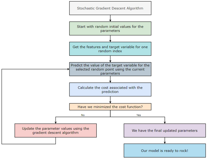
随机梯度下降 (SGD) 算法的工作原理
在批量梯度下降算法中,我们考虑算法所有迭代的所有训练示例。但是,如果我们的数据集有大量训练示例和/或特征,那么计算参数值的计算量就会很大。我们知道如果我们为机器学习算法提供更多训练示例,它会产生更高的准确性。但是,随着数据集大小的增加,与之相关的计算量也会增加。让我们举个例子来更好地理解这一点。
批量梯度下降 (BGD)
每次迭代的训练示例数 = 100 万 = 1⁰⁶
迭代次数 = 1000 = 1⁰³
要训练的参数数 = 10000 = 1⁰⁴
总计算量 = 1⁰⁶*1⁰³*1⁰⁴=1⁰¹³
现在,如果我们看上面的数字,它并没有给我们很好的共鸣!所以我们可以说使用Batch Gradient Descent算法看起来效率不高。因此,为了解决这个问题,我们使用随机梯度下降 (SGD) 算法。“Stochastic”这个词的意思是随机的。因此,我们不是对数据集的所有训练示例进行计算,而是随机抽取一个示例并对其进行计算。听起来很有趣,不是吗?我们只考虑随机梯度下降 (SGD) 算法中每次迭代的一个训练示例。让我们看看随机梯度下降基于它的计算有多有效。
随机梯度下降(SGD):
每次迭代的训练示例数 = 1
迭代次数 = 1000 = 1⁰³
要训练的参数数 = 10000 = 1⁰⁴
总计算量 = 1 * 1⁰³*1⁰⁴=1⁰⁷与批量梯度下降的比较:
BGD 中的
总计算量 = 1⁰¹³ SGD 中的总计算量 = 1⁰⁷
**评估:**在此示例中,SGD 比 BGD 快 ¹⁰⁶ 倍。
**注意:**请注意,我们的成本函数不一定会下降,因为我们每次迭代只取一个随机训练样本,所以不要担心。然而,随着我们执行越来越多的迭代,成本函数将逐渐减小。
现在,让我们看看随机梯度下降 (SGD) 算法是如何实现的。
1. 第 1 步:
首先,我们从 GitHub 存储库下载数据文件。
#Fetch the data file from GitHub repository:
!wget https://raw.githubusercontent.com/Pratik-Shukla-22/Gradient-Descent/main/Advertising.csv
从 GitHub 获取数据文件
2. 第 2 步:
接下来,我们将导入一些必需的库来读取、操作和可视化数据。
#Import the required libraries:
import pandas as pd
import numpy as np
import matplotlib.pyplot as plt
导入所需的库
3. 第 3 步:
接下来,我们正在读取数据文件,然后打印它的前五行。
#Read the data file:
data = pd.read_csv("Advertising.csv")
data.head()

#Output:
index,Unnamed: 0,TV,radio,newspaper,sales
0,1,230.1,37.8,69.2,22.1
1,2,44.5,39.3,45.1,10.4
2,3,17.2,45.9,69.3,9.3
3,4,151.5,41.3,58.5,18.5
4,5,180.8,10.8,58.4,12.9
读取和打印数据
4. 第 4 步:
接下来,我们将数据集划分为特征和目标变量。
获取特征和目标变量
#Define the feature and target variables:
X = data[[“TV”,“radio”,“newspaper”]]
Y = data[“sales”]
尺寸:X = (200, 3) & Y = (200, )
5. 第 5 步:
为了在进一步的步骤中执行矩阵计算,我们需要重塑目标变量。
#Reshape the data in Y:
Y = np.asarray(Y)
Y = np.reshape(Y,(Y.shape[0],1))
重塑 Y 中的数据
尺寸:X = (200, 3) & Y = (200, 1)
6. 第 6 步:
接下来,我们正在规范化数据集。
#Normalize the data:
X = (X - X.mean())/X.std()
Y = Y - Y.mean()/Y.std()
规范化数据
尺寸:X = (200, 3) & Y = (200, 1)
7. 第 7 步:
接下来,我们获取bias和weights矩阵的初始值。我们将在执行前向传播时在第一次迭代中使用这些值。
#Function to get intial weights and bias:
def initialize_weights(n_features):
  bias = np.random.random(1)
  weights = np.random.random(n_features)

  #Reshape the bias and weights:
  bias = np.reshape(bias,(1,1))
  weights = np.reshape(weights, (1,X.shape[1]))

  return bias,weights
获取随机值来初始化我们的参数
维度:偏差 = (1, 1) & 权重 = (1, 3)
8. 第 8 步:
接下来,我们执行前向传播步骤。此步骤基于以下公式。
[外链图片转存失败,源站可能有防盗链机制,建议将图片保存下来直接上传(img-xb7ffmRL-1675607790976)(null)]
预测目标变量的值
#Predict the value of target variable based on the random weights:
def predict(bias, weights, X):
  predicted_value = bias+np.dot(X,weights.T)
  return predicted_value
维度:预测值 = (1, 1)+(200, 3)*(3,1) = (1, 1)+(200, 1) = (200, 1)
9. 第 9 步:
接下来,我们将计算与我们的预测相关的成本。用于此步骤的公式如下。因为只有一个误差值,所以我们不需要将成本函数除以数据集的大小或将所有成本值相加。
[外链图片转存失败,源站可能有防盗链机制,建议将图片保存下来直接上传(img-uAFsiQV9-1675607790950)(null)]
#Calculate the cost:
def calculate_cost(Y, Y_pred):
  error = Y_pred - Y
  cost = np.sum((error)**2)
  return cost
获取与预测相关的成本
维度:成本 = 标量值
10. 第 10 步:
接下来,我们使用梯度下降算法更新权重和偏差的参数值。此步骤基于以下公式。请注意,我们不对权重值求和的原因是我们的权重矩阵不是1*1矩阵。此外,在这种情况下,由于我们只有一个训练示例,因此我们不需要对所有示例执行求和。更新后的公式如下。
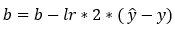
[外链图片转存失败,源站可能有防盗链机制,建议将图片保存下来直接上传(img-PFE0tZ1b-1675607791000)(null)]
#Update the parameter values:
def update_parameters(X,Y,Y_pred,bias,weights,lr):
  #Calculating the gradients:
  db = (Y_pred-Y)*2
  dw = np.dot((Y_pred-Y).T,X)*2

  #Updating the parameters:
  bias = bias - lr*db
  weights = weights - lr*dw

  #Return the updated parameters:
  return bias, weights
使用梯度下降算法更新参数
维度:db = (1, 1)
维度:dw = (1, 200) * (200, 3) = (1, 3)
维度:偏差 = (1, 1) & 权重 = (1, 3)
11. 第 11 步:
随机梯度下降算法
#The main function to run the gradient descent algorithm:
def run_stochastic_gradient_descent(X,Y,lr,iter):
  #Create an empty list to store cost values:
  cost_list = []

  #Get the initial values of weights and bias:
  bias, weights = initialize_weights(X.shape[1])

  for i in range(iter):
    #Get a random index:
    random_index = np.random.randint(0,len(X))

    #Get the X values of the random index:
    X_sample = X.iloc[random_index]
    #Get the Y values of the random index:
    Y_sample = Y[random_index]

    #Reshaping the data:
    X_sample = np.asarray(X_sample)
    X_sample = np.reshape(X_sample,(1,3))

    #Predict the value of the target variable:
    Y_pred = predict(bias, weights, X_sample)

    #Calculate the cost associated with prediction:
    cost = calculate_cost(Y_sample, Y_pred)

    #Append the cost to the list:
    cost_list.append(cost)

    #Update the parameters using gradient descent:
    bias, weights = update_parameters(X_sample,Y_sample,Y_pred,bias,weights,lr)

  #Return the cost list:
  return bias,weights,cost_list
12. 第 12 步:
接下来,我们实际上是在调用函数来获取最终结果。请注意,我们运行的是200 iterations. 此外,我们在这里指定了learning rate of 0.01.
#Run the gradient descent algorithm:
bias,weights,cost = run_stochastic_gradient_descent(X,Y,lr=0.01,iter=200)
运行随机梯度下降算法 200 次迭代
13. 第 13 步:
接下来,我们在final weights完成所有迭代后打印值。
#Print the final values of weights:
print("Weights=",weights)

#Output:
Weights= [[3.90559756 2.84287236 0.26057117]]
在 200 次迭代后打印权重的最终值
14. 第 14 步:
接下来,我们在final bias完成所有迭代后打印值。
#Print the final value of bias:
print("Bias=",bias)

#Output:
Bias= [[11.07422092]]
在 200 次迭代后打印偏差的最终值
15. 第 15 步:
接下来,我们正在绘制 的图形iterations vs. cost。
#Plot the graph of iter. vs cost:
plt.title("Iterations vs. Cost")
plt.xlabel("Iterations")
plt.ylabel("MSE cost")
plt.plot(cost)
plt.plot(cost,label="Stochastic Gradient Descent")
plt.legend()
plt.show()
[外链图片转存失败,源站可能有防盗链机制,建议将图片保存下来直接上传(img-Xf9gxbv3-1675607790928)(null)]
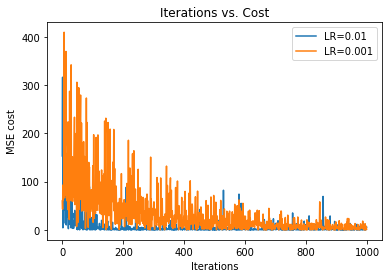
16. 第 16 步:
接下来,我们绘制两个具有不同学习率的图,以查看学习率在优化中的影响。在下图中,我们可以看到学习率较高(0.01)的图比学习率较慢的图收敛得更快(0.001)。同样,我们知道这一点是因为学习率较低的图采用较小的步长。
#Run the gradient descent algorithm:
bias1, weights1, cost1 = run_stochastic_gradient_descent(X,Y,lr=0.01,iter=1000)
bias2, weights2, cost2 = run_stochastic_gradient_descent(X,Y,lr=0.001,iter=1000)

#Plot the graphs:
plt.title("Iterations vs. Cost")
plt.xlabel("Iterations")
plt.ylabel("MSE cost")
plt.plot(cost1,label="LR=0.01")
plt.plot(cost2,label="LR=0.001")
plt.legend()
plt.show()
绘制不同学习率的批量梯度下降算法图
17. 第 17 步:
把它们放在一起。
#Fetch the data file from GitHub repository:
!wget https://raw.githubusercontent.com/Pratik-Shukla-22/Gradient-Descent/main/Advertising.csv

#Import the required libraries:
import pandas as pd
import numpy as np
import matplotlib.pyplot as plt

#Read the data file:
data = pd.read_csv("Advertising.csv")
print(data.head())

#Define the feature and target variables:
X = data[["TV","radio","newspaper"]]
Y = data["sales"]

#Reshape the data in Y:
Y = np.asarray(Y)
Y = np.reshape(Y,(Y.shape[0],1))

#Normalize the data:
X = (X - X.mean())/X.std()
Y = Y - Y.mean()/Y.std()

#Function to get intial weights and bias:
def initialize_weights(n_features):
  bias = np.random.random(1)
  weights = np.random.random(n_features)

  #Reshape the bias and weights:
  bias = np.reshape(bias,(1,1))
  weights = np.reshape(weights, (1,X.shape[1]))

  return bias,weights

#Predict the value of target variable based on the random weights:
def predict(bias, weights, X):
  predicted_value = bias+np.dot(X,weights.T)
  return predicted_value

#Calculate the cost:
def calculate_cost(Y, Y_pred):
  error = Y_pred - Y
  cost = np.sum((error)**2)
  return cost

#Update the parameter values:
def update_parameters(X,Y,Y_pred,bias,weights,lr):
  #Calculating the gradients:
  db = (Y_pred-Y)*2
  dw = np.dot((Y_pred-Y).T,X)*2

  #Updating the parameters:
  bias = bias - lr*db
  weights = weights - lr*dw

  #Return the updated parameters:
  return bias, weights

#The main function to run the gradient descent algorithm:
def run_stochastic_gradient_descent(X,Y,lr,iter):
  #Create an empty list to store cost values:
  cost_list = []

  #Get the initial values of weights and bias:
  bias, weights = initialize_weights(X.shape[1])

  for i in range(iter):
    #Get a random index:
    random_index = np.random.randint(0,len(X))

    #Get the X values of the random index:
    X_sample = X.iloc[random_index]
    #Get the Y values of the random index:
    Y_sample = Y[random_index]

    #Reshaping the data:
    X_sample = np.asarray(X_sample)
    X_sample = np.reshape(X_sample,(1,3))

    #Predict the value of the target variable:
    Y_pred = predict(bias, weights, X_sample)

    #Calculate the cost associated with prediction:
    cost = calculate_cost(Y_sample, Y_pred)

    #Append the cost to the list:
    cost_list.append(cost)

    #Update the parameters using gradient descent:
    bias, weights = update_parameters(X_sample,Y_sample,Y_pred,bias,weights,lr)

  #Return the cost list:
  return bias,weights,cost_list

#Run the gradient descent algorithm:
bias,weights,cost = run_stochastic_gradient_descent(X,Y,lr=0.01,iter=200)

#Print the final values of weights:
print("Weights=",weights)

#Print the final value of bias:
print("Bias=",bias)

#Plot the graph of iter. vs cost:
plt.title("Iterations vs. Cost")
plt.xlabel("Iterations")
plt.ylabel("MSE cost")
plt.plot(cost)
plt.plot(cost,label="Stochastic Gradient Descent")
plt.legend()
plt.show()

#Run the gradient descent algorithm:
bias1, weights1, cost1 = run_stochastic_gradient_descent(X,Y,lr=0.01,iter=1000)
bias2, weights2, cost2 = run_stochastic_gradient_descent(X,Y,lr=0.001,iter=1000)

#Plot the graphs:
plt.title("Iterations vs. Cost")
plt.xlabel("Iterations")
plt.ylabel("MSE cost")
plt.plot(cost1,label="LR=0.01")
plt.plot(cost2,label="LR=0.001")
plt.legend()
plt.show()
计算:
现在,让我们统计一下在实现批量梯度下降算法时执行的计算次数。
**偏差:(**训练示例)x(迭代)x(参数)= 1* 200 * 1 = 200
**权重:(**训练样例)x(迭代次数)x(参数)= 1* 200 *3 = 600
源码:
以上所有代码请关注wx: 猛男技术控
回复梯度下降 即可获取