一、CE Loss
定义
交叉熵损失(Cross-Entropy Loss,CE Loss)能够衡量同一个随机变量中的两个不同概率分布的差异程度,当两个概率分布越接近时,交叉熵损失越小,表示模型预测结果越准确。
公式
二分类
二分类的CE Loss公式如下,
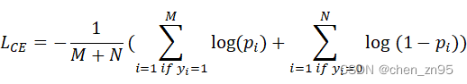
其中,:正样本数量,
:负样本数量,
:真实值,
:预测值
多分类
在计算多分类的CE Loss时,首先需要对模型输出结果进行softmax处理。公式如下,
![]()

其中, :模型输出,
:对模型输出进行softmax处理后的值,
![]() :真实值的one hot编码(假设模型在做5分类,如果
:真实值的one hot编码(假设模型在做5分类,如果=2,则
![]() =[0,0,1,0,0])
=[0,0,1,0,0])
代码实现
二分类
import torch
import torch.nn as nn
import math

criterion = nn.BCELoss()
output = torch.rand(1, requires_grad=True)
label = torch.randint(0, 1, (1,)).float()
loss = criterion(output, label)

print("预测值:", output)
print("真实值:", label)
print("nn.BCELoss:", loss)

for i in range(label.shape[0]):
    if label[i] == 0:
        res = -math.log(1-output[i])
    elif label[i] == 1:
        res = -math.log(output[i])
print("自己的计算结果", res)


"""
预测值: tensor([0.7359], requires_grad=True)
真实值: tensor([0.])
nn.BCELoss: tensor(1.3315, grad_fn=<BinaryCrossEntropyBackward0>)
自己的计算结果 1.331509556677378
"""
多分类
import torch
import torch.nn as nn
import math

criterion = nn.CrossEntropyLoss()
output = torch.randn(1, 5, requires_grad=True)
label = torch.empty(1, dtype=torch.long).random_(5)
loss = criterion(output, label)

print("预测值:", output)
print("真实值:", label)
print("nn.CrossEntropyLoss:", loss)

output = torch.softmax(output, dim=1)
print("softmax后的预测值:", output)

one_hot = torch.zeros_like(output).scatter_(1, label.view(-1, 1), 1)
print("真实值对应的one_hot编码", one_hot)

res = (-torch.log(output) * one_hot).sum()
print("自己的计算结果", res)


"""
预测值: tensor([[-0.7459, -0.3963, -1.8046,  0.6815,  0.2965]], requires_grad=True)
真实值: tensor([1])
nn.CrossEntropyLoss: tensor(1.9296, grad_fn=<NllLossBackward0>)
softmax后的预测值: tensor([[0.1024, 0.1452, 0.0355, 0.4266, 0.2903]], grad_fn=<SoftmaxBackward0>)
真实值对应的one_hot编码 tensor([[0., 1., 0., 0., 0.]])
自己的计算结果 tensor(1.9296, grad_fn=<SumBackward0>)
"""
二、Focal Loss
定义
虽然CE Loss能够衡量同一个随机变量中的两个不同概率分布的差异程度,但无法解决以下两个问题:1、正负样本数量不平衡的问题(如centernet的分类分支,它只将目标的中心点作为正样本,而把特征图上的其它像素点作为负样本,可想而知正负样本的数量差距之大);2、无法区分难易样本的问题(易分类的样本的分类错误的损失占了整体损失的绝大部分,并主导梯度)
为了解决以上问题,Focal Loss在CE Loss的基础上改进,引入了:1、正负样本数量调节因子以解决正负样本数量不平衡的问题;2、难易样本分类调节因子以聚焦难分类的样本
公式
二分类
公式如下,

![]()

其中,:正负样本数量调节因子,
:难易样本分类调节因子
多分类

其中,:
类别的权重
代码实现
二分类
def sigmoid_focal_loss(
    inputs: torch.Tensor,
    targets: torch.Tensor,
    alpha: float = -1,
    gamma: float = 2,
    reduction: str = "none",
) -> torch.Tensor:
    """
    Loss used in RetinaNet for dense detection: https://arxiv.org/abs/1708.02002.
    Args:
        inputs: A float tensor of arbitrary shape.
                The predictions for each example.
        targets: A float tensor with the same shape as inputs. Stores the binary
                 classification label for each element in inputs
                (0 for the negative class and 1 for the positive class).
        alpha: (optional) Weighting factor in range (0,1) to balance
                positive vs negative examples. Default = -1 (no weighting).
        gamma: Exponent of the modulating factor (1 - p_t) to
               balance easy vs hard examples.
        reduction: 'none' | 'mean' | 'sum'
                 'none': No reduction will be applied to the output.
                 'mean': The output will be averaged.
                 'sum': The output will be summed.
    Returns:
        Loss tensor with the reduction option applied.
    """
    inputs = inputs.float()
    targets = targets.float()
    p = torch.sigmoid(inputs)
    ce_loss = F.binary_cross_entropy_with_logits(inputs, targets, reduction="none")
    p_t = p * targets + (1 - p) * (1 - targets)
    loss = ce_loss * ((1 - p_t) ** gamma)

    if alpha >= 0:
        alpha_t = alpha * targets + (1 - alpha) * (1 - targets)
        loss = alpha_t * loss

    if reduction == "mean":
        loss = loss.mean()
    elif reduction == "sum":
        loss = loss.sum()

    return loss
步骤1、首先对输入进行sigmoid处理,
p = torch.sigmoid(inputs)步骤2、随后求出CE Loss,
ce_loss = F.binary_cross_entropy_with_logits(inputs, targets, reduction="none")步骤3、定义,公式为:
p_t = p * targets + (1 - p) * (1 - targets)步骤4、为CE Loss添加难易样本分类调节因子,
loss = ce_loss * ((1 - p_t) ** gamma)步骤5、定义,公式为:
![]()
alpha_t = alpha * targets + (1 - alpha) * (1 - targets)步骤6、为步骤4的损失添加正负样本数量调节因子,
loss = alpha_t * loss多分类
def multi_cls_focal_loss(
    inputs: torch.Tensor,
    targets: torch.Tensor,
    alpha: torch.Tensor,
    gamma: float = 2,
    reduction: str = "none",
) -> torch.Tensor:

    inputs = inputs.float()
    targets = targets.float()
    ce_loss = nn.CrossEntropyLoss()(inputs, targets, reduction="none")
    one_hot = torch.zeros_like(inputs).scatter_(1, targets.view(-1, 1), 1)
    p_t = inputs * one_hot
    loss = ce_loss * ((1 - p_t) ** gamma)

    if alpha >= 0:
        alpha_t = alpha * one_hot
        loss = alpha_t * loss

    return loss
三、GHMC Loss
定义
Focal Loss在CE Loss的基础上改进后,解决了正负样本不平衡以及无法区分难易样本的问题,但也会过分关注难分类的样本(离群点),导致模型学歪。为了解决这个问题,GHMC(Gradient Harmonizing Mechanism-C)定义了梯度模长,该梯度模长正比于分类的难易程度,目的是让模型不要关注那些容易学的样本,也不要关注那些特别难分的样本
公式
1、定义梯度模长
二分类的CE Loss公式如下,

假设x是模型的输出,假设p=sigmoid(x),求损失对x的偏导,
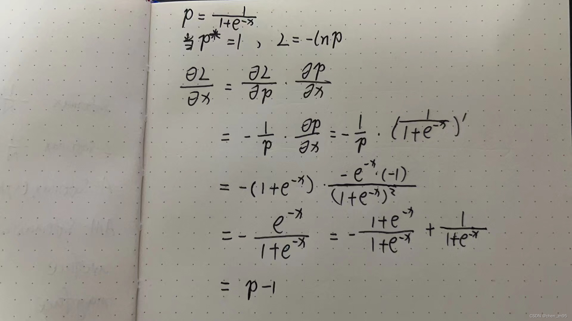

因此,定义梯度模长如下,

其中, :预测值,
:真实值
梯度模长与样本数量的关系如下,

2、定义梯度密度(单位梯度模长g上的样本数量)


其中,:第k个样本的梯度模长,
:
在
范围内的样本数量,
:区间
的长度
3、定义梯度密度协调参数(gradient density harmonizing parameter)

其中,:样本总数
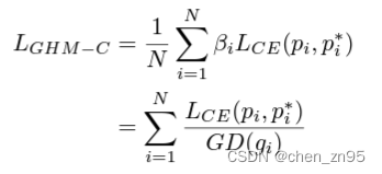
4、定义GHMC Loss
代码实现
def _expand_binary_labels(labels, label_weights, label_channels):
    bin_labels = labels.new_full((labels.size(0), label_channels), 0)
    inds = torch.nonzero(labels >= 1).squeeze()
    if inds.numel() > 0:
        bin_labels[inds, labels[inds] - 1] = 1
    bin_label_weights = label_weights.view(-1, 1).expand(
        label_weights.size(0), label_channels)
    return bin_labels, bin_label_weights


class GHMC(nn.Module):
    def __init__(
            self,
            bins=10,
            momentum=0,
            use_sigmoid=True,
            loss_weight=1.0):
        super(GHMC, self).__init__()
        self.bins = bins
        self.momentum = momentum
        self.edges = [float(x) / bins for x in range(bins+1)]
        self.edges[-1] += 1e-6
        if momentum > 0:
            self.acc_sum = [0.0 for _ in range(bins)]
        self.use_sigmoid = use_sigmoid
        self.loss_weight = loss_weight

    def forward(self, pred, target, label_weight, *args, **kwargs):
        """ Args:
        pred [batch_num, class_num]:
            The direct prediction of classification fc layer.
        target [batch_num, class_num]:
            Binary class target for each sample.
        label_weight [batch_num, class_num]:
            the value is 1 if the sample is valid and 0 if ignored.
        """
        if not self.use_sigmoid:
            raise NotImplementedError
        # the target should be binary class label
        if pred.dim() != target.dim():
            target, label_weight = _expand_binary_labels(target, label_weight, pred.size(-1))
        target, label_weight = target.float(), label_weight.float()
        edges = self.edges
        mmt = self.momentum
        weights = torch.zeros_like(pred)

        # 计算梯度模长
        g = torch.abs(pred.sigmoid().detach() - target)

        valid = label_weight > 0
        tot = max(valid.float().sum().item(), 1.0)

        # 设置有效区间个数
        n = 0
        for i in range(self.bins):
            inds = (g >= edges[i]) & (g < edges[i+1]) & valid
            num_in_bin = inds.sum().item()
            if num_in_bin > 0:
                if mmt > 0:
                    self.acc_sum[i] = mmt * self.acc_sum[i] \
                        + (1 - mmt) * num_in_bin
                    weights[inds] = tot / self.acc_sum[i]
                else:
                    weights[inds] = tot / num_in_bin
                n += 1
        if n > 0:
            weights = weights / n

        loss = F.binary_cross_entropy_with_logits(
            pred, target, weights, reduction='sum') / tot
        return loss * self.loss_weight
步骤一、将梯度模长划分为bins(默认为10)个区域,
self.edges = [float(x) / bins for x in range(bins+1)]
"""
[0.0000, 0.1000, 0.2000, 0.3000, 0.4000, 0.5000, 0.6000, 0.7000, 0.8000, 0.9000, 1.0000]
"""
步骤二、计算梯度模长
g = torch.abs(pred.sigmoid().detach() - target)步骤三、计算落入不同bin区间的梯度模长数量
valid = label_weight > 0
tot = max(valid.float().sum().item(), 1.0)
n = 0
for i in range(self.bins):
    inds = (g >= edges[i]) & (g < edges[i+1]) & valid
    num_in_bin = inds.sum().item()
    if num_in_bin > 0:
        if mmt > 0:
            self.acc_sum[i] = mmt * self.acc_sum[i] + (1 - mmt) * num_in_bin
            weights[inds] = tot / self.acc_sum[i]
        else:
            weights[inds] = tot / num_in_bin
        n += 1
if n > 0:
    weights = weights / n
步骤四、计算GHMC Loss
loss = F.binary_cross_entropy_with_logits(pred, target, weights, reduction='sum') / tot * self.loss_weight
【参考文章】
Focal Loss的理解以及在多分类任务上的使用(Pytorch)_focal loss 多分类_GHZhao_GIS_RS的博客-CSDN博客