转自:https://blog.csdn.net/qq_34564947/article/details/77200104
Focal Loss for Dense Object Detection
引入问题
目前目标检测的框架一般分为两种:基于候选区域的two-stage的检测框架(比如fast r-cnn系列),基于回归的one-stage的检测框架(yolo,ssd这种),two-stage的效果好,one-stage的快但是效果差一些。
本文作者希望弄明白为什么one-stage的检测器准确率不高的问题,作者给出的解释是由于前正负样本不均衡的问题(感觉理解成简单-难分样本不均衡比较好)
We discover that the extreme foreground-background class imbalance encountered during training of dense detectors is the central cause
样本的类别不均衡会带来什么问题
(1) training is inefficient as most locations are easy negatives that contribute no useful learning signal;
(2) en masse,the easy negatives can overwhelm training and lead to degenerate models.
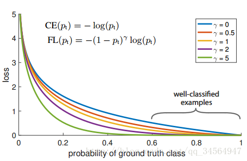
由于大多数都是简单易分的负样本(属于背景的样本),使得训练过程不能充分学习到属于那些有类别样本的信息;其次简单易分的负样本太多,可能掩盖了其他有类别样本的作用(这些简单易分的负样本仍产生一定幅度的loss,见下图蓝色曲线,数量多会对loss起主要贡献作用,因此就主导了梯度的更新方向,掩盖了重要的信息)
对于two-stage的检测器而言,通常分为两个步骤,第一个步骤即产生合适的候选区域,而这些候选区域经过筛选,一般控制一个比例(比如正负样本1:3),另外还通过hard negatiive mining(OHEM),控制难分样本占据的比例,以解决样本类别不均衡的问题。
对于one-stage的检测器来说,尽管可以采用同样的策略(OHEM)控制正负样本,但是还是有缺陷,文中的说法是:
Like the focal loss,OHEM puts more emphasis on misclassified examples, but unlike FL, OHEM completely discards easy examples
While similar sampling heuristics may also be applied, they are inefficient as the training procedure is still dominated by easily classified background examples
OHEM这篇论文还没看,所以不是特别理解。
所以作者提出Focal loss,基于损失函数做出改进。
解决方案:Focal Loss
作者提出一种新的损失函数,思路是希望那些hard examples对损失的贡献变大,使网络更倾向于从这些样本上学习。
作者以二分类为例进行说明:
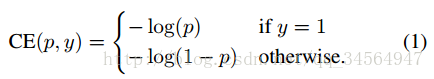
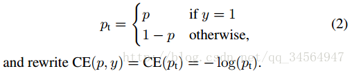
首先是我们常使用的交叉熵损失函数:
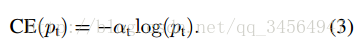
要对类别不均衡问题对loss的贡献进行一个控制,即加上一个控制权重即可,最初作者的想法即如下这样,对于属于少数类别的样本,增大α即可
但这样有一个问题,它仅仅解决了正负样本之间的平衡问题,并没有区分易分/难分样本,按作者的话说:
Easily classified negatives comprise the majority of the loss and dominate the gradient.
While α balances the importance of positive/negative examples, it does not differentiate between easy/hard examples.
因此后面有了如下的形式:
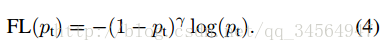
显然,样本越易分,pt越大,则贡献的loss就越小,相对来说,难分样本所占的比重就会变大,见如下原文中的一个例子:
For instance, with γ = 2, an example classified with pt = 0:9 would have 100× lower loss compared with CE and with pt ≈ 0:968 it would have 1000× lower loss. This in turn increases the importance of correcting misclassified examples (whose loss is scaled down by at most 4× for pt ≤ .5 and γ = 2)
因此,通过这个公式区分了易分/难分样本,在实际中,作者采用如下公式,即综合了上述两个公式的形式:
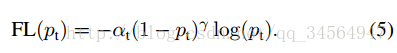
这里的两个参数α和γ协调来控制,本文作者采用α=0.25,γ=2效果最好
另外:作者提到了类别不均衡和模型的初始化问题,即数量很多的某一类样本会起主导作用,在开始训练的时候可能导致不稳定,作者提出的解决方法是:
To counter this, we introduce the concept of a ‘prior’ for the value of p estimated by the model for the rare class (foreground) at the start of training.
For the final conv
layer of the classification subnet, we set the bias initialization to b = − log((1 − π)=π), where π specifies that at the start of training every anchor should be labeled as foreground with confidence of ∼π.
π采用的是0.01,不太清楚为什么要这么做,留个问号,help
实验框架
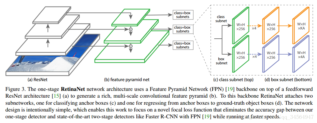
本文作者实验时设计了一个叫RetinaNet的one-satge的网络结构,以证明通过Focal Loss,one-stage的网络结构也能够达到two-stage的准确率,实际上采用的是基于resnet的FPN(特征金字塔网络,可自行查阅论文论文链接),网络框架如下:
实验结果
最好能在coco test-dev上达到 39.1AP,5Fps
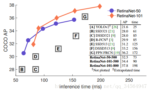
由上图可见,准确率高于two-stage的方法,并且速度可以得到保持
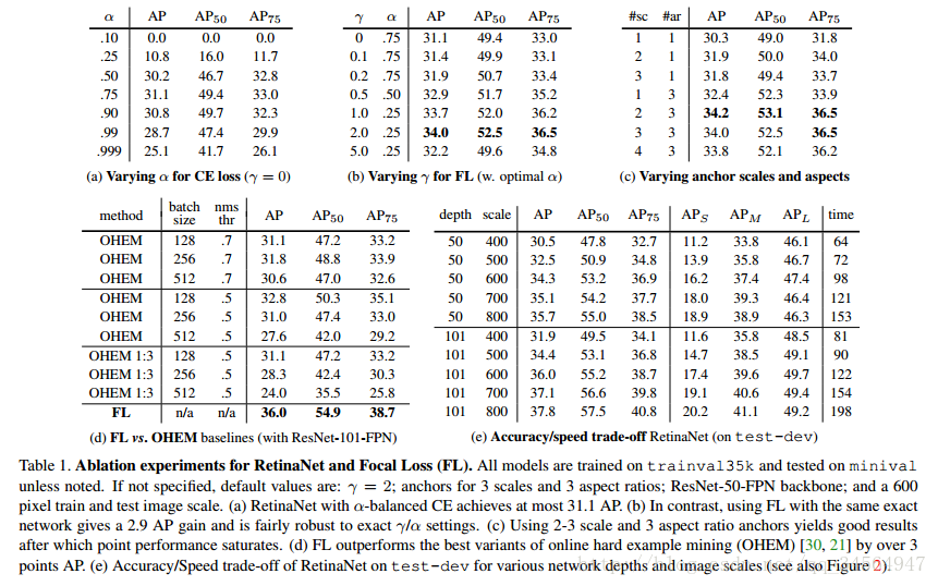
上图是各指标的对比实验结果,具体可查看论文
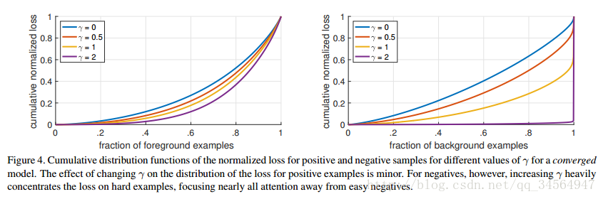
上图表明了该loss对负样本的影响很明显,使得负样本的loss集中在少数的样本上:
As can be seen, FL can effectively discount the effect of easy negatives, focusing all attention on the hard negative examples.
另外Focal loss的形式并不一定要是公式那样的形式,只要能够发挥相同的作用即可,作者有实验证明,具体可查阅论文。
结论
本文从loss的角度阐述了one-stage检测器准确率低的问题,并给出了解决方案,很精彩。