高编课后作业------第十四周-Scipy exercise

上一篇博客应该是13周，上次打错了，已纠正。

用jupyter写完可以直接生成 markdown，然后复制过来就行了，挺方便的

%matplotlib inline

import random

import numpy as np
import scipy as sp
import pandas as pd
import matplotlib.pyplot as plt
import seaborn as sns

import statsmodels.api as sm
import statsmodels.formula.api as smf

sns.set_context("talk")

Anscombe’s quartet

Anscombe’s quartet comprises of four datasets, and is rather famous. Why? You’ll find out in this exercise.

anascombe = pd.read_csv('C:/Users/sunyy/Desktop/cme193-ipython-notebooks-lecture-master/data/anscombe.csv')
anascombe.head()

.dataframe tbody tr th:only-of-type { vertical-align: middle; } .dataframe tbody tr th { vertical-align: top; } .dataframe thead th { text-align: right; }

	dataset	x	y
0	I	10.0	8.04
1	I	8.0	6.95
2	I	13.0	7.58
3	I	9.0	8.81
4	I	11.0	8.33

计算均值

print(anascombe.groupby('dataset')['x'].mean())
print(anascombe.groupby('dataset')['y'].mean())

dataset
I      9.0
II     9.0
III    9.0
IV     9.0
Name: x, dtype: float64
dataset
I      7.500909
II     7.500909
III    7.500000
IV     7.500909
Name: y, dtype: float64

计算方差

print(anascombe.groupby('dataset')['x'].var())
print(anascombe.groupby('dataset')['y'].var())

dataset
I      11.0
II     11.0
III    11.0
IV     11.0
Name: x, dtype: float64
dataset
I      4.127269
II     4.127629
III    4.122620
IV     4.123249
Name: y, dtype: float64

相关系数不好直接用groupby分组算，所以先手动获取每组数据

Y1 = anascombe.y[0:10].values  
Y2 = anascombe.y[11:21].values  
Y3 = anascombe.y[22:32].values  
Y4 = anascombe.y[33:43].values  
X1 = anascombe.x[0:10].values  
X2 = anascombe.x[11:21].values  
X3 = anascombe.x[22:32].values  
X4 = anascombe.x[33:43].values 

计算相关系数

cof = [0,0,0,0]
cof[0] = sp.stats.pearsonr(X1, Y1)[0]  #返回的第一个参数是相关系数
cof[1] = sp.stats.pearsonr(X2, Y2)[0]  
cof[2] = sp.stats.pearsonr(X3, Y3)[0]  
cof[3] = sp.stats.pearsonr(X4, Y4)[0] 
for co in cof:
    print(co)

0.7970815759062526
0.7773093020784241
0.7985632617088811
0.8146722146933596

线性回归

执行过程大概分成3步：
X=sm.add_constant(X)  #为模型增加常数项
est=sm.OLS(Y,X)
est=est.fit()
est.params
params 里包括了 前2个系数 ，第三个是误差项

X1add=sm.add_constant(X1)  #为模型增加常数项
est=sm.OLS(Y1,X1add)
est=est.fit()
print("For dataset I, β0 is " + str(est.params[0]) + " ,  β1 is" + str(est.params[1]))
X2add=sm.add_constant(X2)  #为模型增加常数项
est=sm.OLS(Y2,X2add)
est=est.fit()
print("For dataset II, β0 is " + str(est.params[0]) + " ,  β1 is" + str(est.params[1]))
X3add=sm.add_constant(X3)  #为模型增加常数项
est=sm.OLS(Y3,X3add)
est=est.fit()
print("For dataset III, β0 is " + str(est.params[0]) + " ,  β1 is" + str(est.params[1]))
X4add=sm.add_constant(X4)  #为模型增加常数项
est=sm.OLS(Y4,X4add)
est=est.fit()
print("For dataset IIII, β0 is " + str(est.params[0]) + " ,  β1 is" + str(est.params[1]))

For dataset I, β0 is 2.9018181818181805 ,  β1 is0.5086363636363642
For dataset II, β0 is 3.417597402597403 ,  β1 is0.46376623376623394
For dataset III, β0 is 2.877099567099566 ,  β1 is0.5106277056277062
For dataset IIII, β0 is 3.023030303030302 ,  β1 is0.49878787878787884

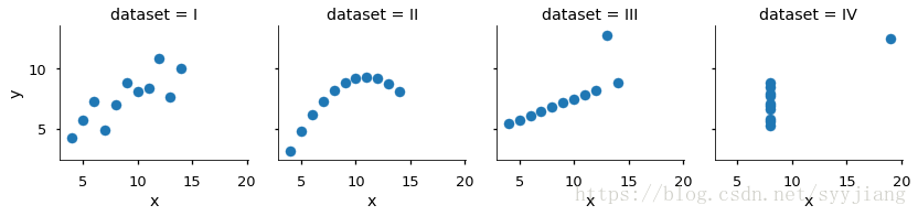
官方的用法就是这样，也没有什么好解释的：

m = sns.FacetGrid(anascombe, col="dataset")    
m.map(plt.scatter, "x","y")