[python 作业] [第十二周] matplotlib exercise

代码：

import numpy as np
import matplotlib.pyplot as plt

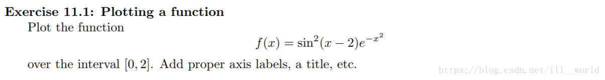
# Exercise 11.1: Plotting a function

x = np.linspace(0, 2, 50)
y = pow(np.sin(x-2), 2) * np.exp(-x**2)
plt.plot(x, y)
plt.xlim((0, 2))    # set the limit of x axis
plt.ylim((0, 1))
plt.xlabel('x')     # set the label of x
plt.ylabel('y = $sin^2$'+'(x-2)'+'$e^-$'+'$^x$'+'$^2$')
plt.title('Exercise 11.1: Plotting a function')

plt.axis('equal') # let the unit length of x and y equal
plt.grid(True)    # drew grids
plt.savefig('Exercise11_1.png') # save the figure as a png file
plt.show()

运行结果：

---

代码：

import numpy as np
import matplotlib.pyplot as plt

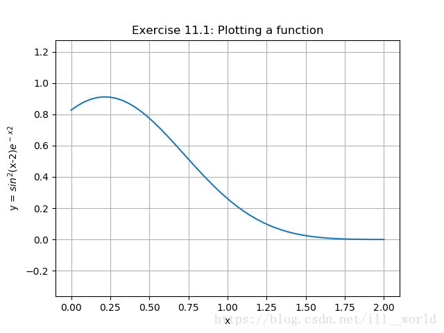
# Exercise 11.2: Data

X = np.random.randn(20, 10) # get a matrix 20 * 10
b = np.random.randn(10, 1)
z = np.random.randn(20, 1)
y = np.dot(X, b) + z

b_e = np.linalg.lstsq(X, y, rcond=None)[0]  # find an estimator for b

plt.scatter(np.arange(10), b_e, color='blue', marker='o', label='True coefficients')    # dram the scatter plot of the True coefficients
plt.scatter(np.arange(10), b, color='red', marker='x', label='Estimated coefficients')  # dram the scatter plot of the Estimated coefficients
plt.xticks(np.arange(10))   # set the index of x from 0 to 9
plt.legend()    
plt.savefig('Exercise11_2.png')
plt.show()

运行结果：

---

代码：

import numpy as np
import matplotlib.pyplot as plt
from scipy.stats import gaussian_kde

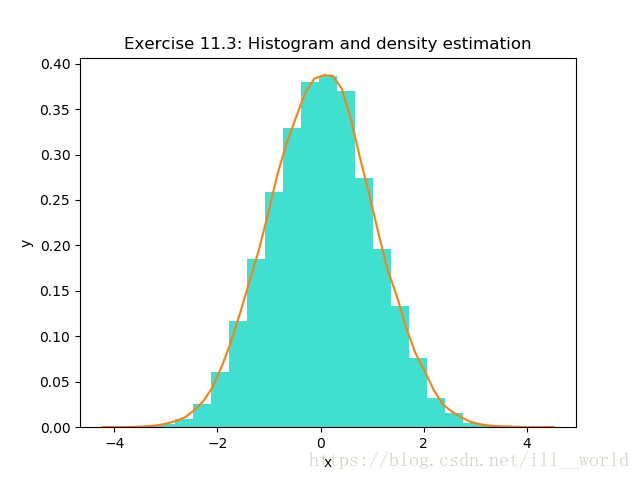
# Exercise 11.3: Histogram and density estimation

observ = 10000
my_bins= 25

z = np.random.normal(size=observ)
x = np.linspace(min(z), max(z), 50)
a = plt.hist(z, bins=my_bins, histtype='bar', facecolor='turquoise', normed=True)
kernel = gaussian_kde(z)

plt.plot(x, kernel.pdf(x)) # pdf = probability density function
plt.title('Exercise 11.3: Histogram and density estimation')
plt.xlabel('x')
plt.ylabel('y')
plt.savefig('Exercise11_3.png')
plt.show()

运行结果：