Exercise: Scipy

Exercise 10.1: Least squares
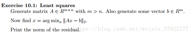
Generate matrix A ∈ Rm × n with m > n. Also generate some vector b ∈ Rm.
Now find x = argminx k Ax − bk 2.

Print the norm of the residual.

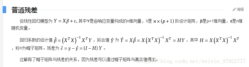
残差定义：

scipy.optimize.lsq_linear

scipy.optimize. lsq_linear ( A,  b,  bounds=(-inf,  inf),  method='trf',  tol=1e-10,  lsq_solver=None,  lsmr_tol=None,  max_iter=None,  verbose=0 ) [source]

Solve a linear least-squares problem with bounds on the variables.

Given a m-by-n design matrix A and a target vector b with m elements, lsq_linear solves the following optimization problem:

minimize 0.5 * ||A x - b||**2
subject to lb <= x <= ub

This optimization problem is convex, hence a found minimum (if iterations have converged) is guaranteed to be global.

Parameters:

A  :  array_like, sparse matrix of LinearOperator, shape (m, n) Design matrix. Can be scipy.sparse.linalg.LinearOperator. b  :  array_like, shape (m,) Target vector. bounds  :  2-tuple of array_like, optional Lower and upper bounds on independent variables. Defaults to no bounds. Each array must have shape (n,) or be a scalar, in the latter case a bound will be the same for all variables. Use np.inf with an appropriate sign to disable bounds on all or some variables. method  :  ‘trf’ or ‘bvls’, optional Method to perform minimization. ‘trf’ : Trust Region Reflective algorithm adapted for a linear least-squares problem. This is an interior-point-like method and the required number of iterations is weakly correlated with the number of variables. ‘bvls’ : Bounded-Variable Least-Squares algorithm. This is an active set method, which requires the number of iterations comparable to the number of variables. Can’t be used when A is sparse or LinearOperator. Default is ‘trf’. tol  :  float, optional Tolerance parameter. The algorithm terminates if a relative change of the cost function is less than tolon the last iteration.  Additionally the first-order optimality measure is considered: method='trf' terminates if the uniform norm of the gradient, scaled to account for the presence of the bounds, is less than tol. method='bvls' terminates if Karush-Kuhn-Tucker conditions are satisfied within tol tolerance. lsq_solver  :  {None, ‘exact’, ‘lsmr’}, optional Method of solving unbounded least-squares problems throughout iterations: ‘exact’ : Use dense QR or SVD decomposition approach. Can’t be used when A is sparse or LinearOperator. ‘lsmr’ : Use scipy.sparse.linalg.lsmr iterative procedure which requires only matrix-vector product evaluations. Can’t be used with method='bvls'. If None (default) the solver is chosen based on type of A. lsmr_tol  :  None, float or ‘auto’, optional Tolerance parameters ‘atol’ and ‘btol’ for scipy.sparse.linalg.lsmr If None (default), it is set to 1e-2 * tol. If ‘auto’, the tolerance will be adjusted based on the optimality of the current iterate, which can speed up the optimization process, but is not always reliable. max_iter  :  None or int, optional Maximum number of iterations before termination. If None (default), it is set to 100 for method='trf' or to the number of variables for method='bvls' (not counting iterations for ‘bvls’ initialization). verbose  :  {0, 1, 2}, optional Level of algorithm’s verbosity: 0 : work silently (default). 1 : display a termination report. 2 : display progress during iterations.

Returns:

OptimizeResult with the following fields defined: x  :  ndarray, shape (n,) Solution found. cost  :  float Value of the cost function at the solution. fun  :  ndarray, shape (m,) Vector of residuals at the solution. optimality  :  float First-order optimality measure. The exact meaning depends on method, refer to the description of tol parameter. active_mask  :  ndarray of int, shape (n,) Each component shows whether a corresponding constraint is active (that is, whether a variable is at the bound): 0 : a constraint is not active. -1 : a lower bound is active. 1 : an upper bound is active. Might be somewhat arbitrary for the trf method as it generates a sequence of strictly feasible iterates and active_mask is determined within a tolerance threshold. nit  :  int Number of iterations. Zero if the unconstrained solution is optimal. status  :  int Reason for algorithm termination: -1 : the algorithm was not able to make progress on the last iteration. 0 : the maximum number of iterations is exceeded. 1 : the first-order optimality measure is less than tol. 2 : the relative change of the cost function is less than tol. 3 : the unconstrained solution is optimal. message  :  str Verbal description of the termination reason. success  :  bool True if one of the convergence criteria is satisfied (status > 0).

numpy.linalg.norm

numpy.linalg. norm ( x,  ord=None,  axis=None,  keepdims=False ) [source]

Matrix or vector norm.

This function is able to return one of eight different matrix norms, or one of an infinite number of vector norms (described below), depending on the value of the ord parameter.

Parameters:

x : array_like Input array. If axis is None, x must be 1-D or 2-D. ord : {non-zero int, inf, -inf, ‘fro’, ‘nuc’}, optional Order of the norm (see table under Notes). inf means numpy’s inf object. axis : {int, 2-tuple of ints, None}, optional If axis is an integer, it specifies the axis of x along which to compute the vector norms. If axis is a 2-tuple, it specifies the axes that hold 2-D matrices, and the matrix norms of these matrices are computed. If axis is None then either a vector norm (when x is 1-D) or a matrix norm (when x is 2-D) is returned. keepdims : bool, optional If this is set to True, the axes which are normed over are left in the result as dimensions with size one. With this option the result will broadcast correctly against the original x. New in version 1.10.0.

Returns:

n : float or ndarray Norm of the matrix or vector(s).

Notes

For values of ord <= 0, the result is, strictly speaking, not a mathematical ‘norm’, but it may still be useful for various numerical purposes.

The following norms can be calculated:

ord	norm for matrices	norm for vectors
None	Frobenius norm	2-norm
‘fro’	Frobenius norm	–
‘nuc’	nuclear norm	–
inf	max(sum(abs(x), axis=1))	max(abs(x))
-inf	min(sum(abs(x), axis=1))	min(abs(x))
0	–	sum(x != 0)
1	max(sum(abs(x), axis=0))	as below
-1	min(sum(abs(x), axis=0))	as below
2	2-norm (largest sing. value)	as below
-2	smallest singular value	as below
other	–	sum(abs(x)**ord)**(1./ord)

程序实现：

import numpy as np
import scipy.optimize as opt

# Exercise 10.1: Least squares
m, n = 100, 50
# Generate matrix A ∈ Rm × n with m > n
A = np.random.rand(m, n)  

# Also generate some vector b ∈ Rm.
b = np.random.random(m)

# Now find x = argminx k Ax − bk 2.
res = opt.lsq_linear(A, b)
x = res.x

# Print the norm of the residual.
residual = b - np.dot(A, x)
norm = np.linalg.norm(residual) #Frobenius norm

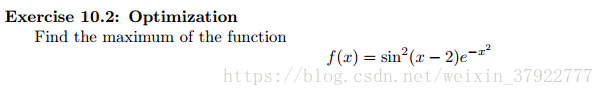
print(norm)

Exercise 10.2: Optimization

Find the maximum of the function

f(x) = sin 2(x − 2)e −x 2

scipy.optimize.minimize_scalar

scipy.optimize. minimize_scalar ( fun,  bracket=None,  bounds=None,  args=(),  method='brent',  tol=None,  options=None ) [source]

Minimization of scalar function of one variable.

Parameters:

fun : callable Objective function. Scalar function, must return a scalar. bracket : sequence, optional For methods ‘brent’ and ‘golden’, bracket defines the bracketing interval and can either have three items (a, b, c) so that a < b < c and fun(b) < fun(a), fun(c) or two items a and c which are assumed to be a starting interval for a downhill bracket search (see bracket); it doesn’t always mean that the obtained solution will satisfy a <= x <= c. bounds : sequence, optional For method ‘bounded’, bounds is mandatory and must have two items corresponding to the optimization bounds. args : tuple, optional Extra arguments passed to the objective function. method : str or callable, optional Type of solver. Should be one of: ‘Brent’ (see here) ‘Bounded’ (see here) ‘Golden’ (see here) custom - a callable object (added in version 0.14.0), see below tol : float, optional Tolerance for termination. For detailed control, use solver-specific options. options : dict, optional A dictionary of solver options. maxiter  :  int Maximum number of iterations to perform. disp  :  bool Set to True to print convergence messages. See show_options for solver-specific options.

Returns:

res : OptimizeResult The optimization result represented as a OptimizeResult object. Important attributes are: x the solution array, success a Boolean flag indicating if the optimizer exited successfully and messagewhich describes the cause of the termination. See OptimizeResult for a description of other attributes.

程序实现：

import numpy as np
import scipy.optimize as opt
# Exercise 10.2: Optimization

# f(x) = sin 2(x − 2)e −x 2
def f(x):  
	res = np.power(np.sin(x-2), 2) * np.exp(-1*(x**2))
	# Change the function into opposite one
	return -1 * res
    
# Find the maximum of the function
res = opt.minimize_scalar(f)
x = res.x
# Equal to find the minimum of the opposite function
print(-1*f(x))

Exercise 10.3: Pairwise distances
Let X be a matrix with n rows and m columns. How can you compute the pairwise distances between
every two rows?

As an example application, consider n cities, and we are given their coordinates in two columns.

Now we want a nice table that tells us for each two cities, how far they are apart.

Again, make sure you make use of Scipy’s functionality instead of writing your own routine.

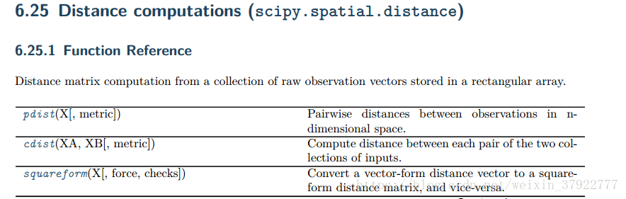
scipy.spatial.distance.pdist

scipy.spatial.distance. pdist ( X,  metric='euclidean',  *args,  **kwargs ) [source]

Pairwise distances between observations in n-dimensional space.

See Notes for common calling conventions.

Parameters:

X  :  ndarray An m by n array of m original observations in an n-dimensional space. metric  :  str or function, optional The distance metric to use. The distance function can be ‘braycurtis’, ‘canberra’, ‘chebyshev’, ‘cityblock’, ‘correlation’, ‘cosine’, ‘dice’, ‘euclidean’, ‘hamming’, ‘jaccard’, ‘kulsinski’, ‘mahalanobis’, ‘matching’, ‘minkowski’, ‘rogerstanimoto’, ‘russellrao’, ‘seuclidean’, ‘sokalmichener’, ‘sokalsneath’, ‘sqeuclidean’, ‘yule’. *args  :  tuple. Deprecated. Additional arguments should be passed as keyword arguments **kwargs  :  dict, optional Extra arguments to metric: refer to each metric documentation for a list of all possible arguments. Some possible arguments: p : scalar The p-norm to apply for Minkowski, weighted and unweighted. Default: 2. w : ndarray The weight vector for metrics that support weights (e.g., Minkowski). V : ndarray The variance vector for standardized Euclidean. Default: var(X, axis=0, ddof=1) VI : ndarray The inverse of the covariance matrix for Mahalanobis. Default: inv(cov(X.T)).T out : ndarray. The output array If not None, condensed distance matrix Y is stored in this array. Note: metric independent, it will become a regular keyword arg in a future scipy version

Returns:

Y  :  ndarray Returns a condensed distance matrix Y. For each i and j (where i<j<m),where m is the number of original observations. The metric dist(u=X[i], v=X[j]) is computed and stored in entry ij.

程序实现：

import numpy as np
import matplotlib.pyplot as plt
from mpl_toolkits.mplot3d import Axes3D
import scipy.spatial.distance as dis
# Exercise 10.3: Pairwise distances

n, m = 50, 100
# Let X be a matrix with n rows and m columns
X = np.random.rand(n, m)

# The first element is dist(X[0], X[1])
# the second is dist(X[0], X[2]) 
# the third is dist(X[0], X[3])
# ...
de = dis.pdist(X)

# As an example application, consider n cities, and we are given their coordinates in two columns
x = []
y = []
for a in range(0, n//2):
	x = x + [a for _ in range(1, n)]
	y = y + [b for b in range(1, n)]

x = np.array(x) # set x lable
y = np.array(y) # set y lable

# Now we want a nice table that tells us for each two cities, how far they are apart.
fig = plt.figure()
ax = Axes3D(fig)

# creat a 3-D table
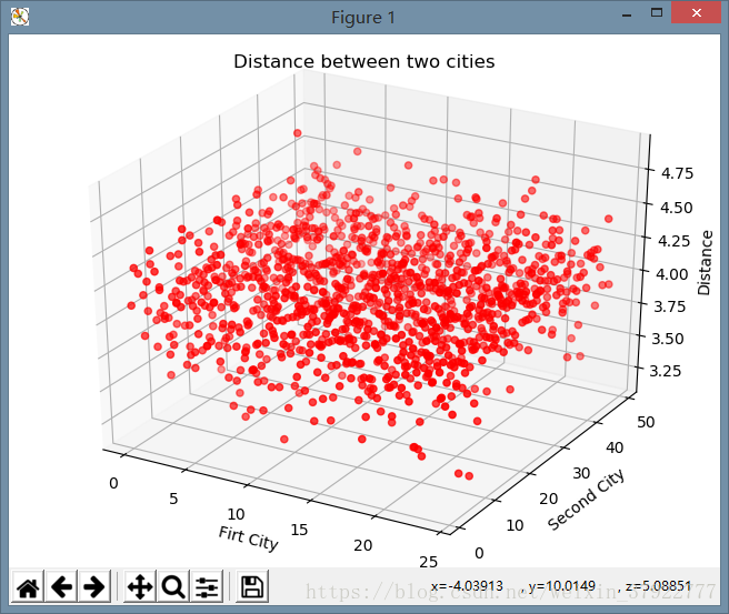
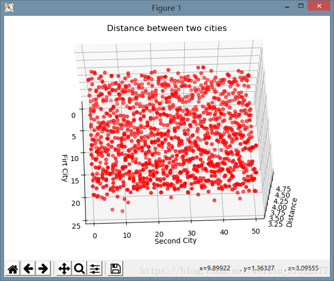
plt.title("Distance between two cities")  
ax.set_xlabel('Firt City')  # 坐标轴
ax.set_ylabel('Second City')
ax.set_zlabel('Distance')

ax.scatter(x, y, de, c='r')
plt.show()

结果显示：