线性回归（skit-learn 实战）

线性回归（skit-learn 实战）

线性回归API

## 引入包

import csv
import numpy as np
import matplotlib.pyplot as plt
import pandas as pd
from sklearn.model_selection import train_test_split
from sklearn.linear_model import LinearRegression
from sklearn.metrics import mean_squared_error
import seaborn as sns

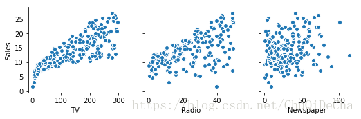
## 数据读取与特征选择 广告投入与销售额数据，共有5列，分别为id，电视广告投入、无限广播投入、报纸投入和销售额。 [下载](https://pan.baidu.com/s/13Foo6dEf2aYqRr2v4NGrfA)

path = './Advertising.csv'

# pandas读入
data = pd.read_csv(path)    # TV、Radio、Newspaper、Sales

data.head()

	Unnamed: 0	TV	Radio	Newspaper	Sales
0	1	230.1	37.8	69.2	22.1
1	2	44.5	39.3	45.1	10.4
2	3	17.2	45.9	69.3	9.3
3	4	151.5	41.3	58.5	18.5
4	5	180.8	10.8	58.4	12.9

# 用pairplot画图，观察Sales与各特征之间的关系
sns.pairplot(data, x_vars=['TV','Radio','Newspaper'], y_vars='Sales')

# 从上图可以看出，Sales与TV具有较强的线性关系，仅选用TV一个feature
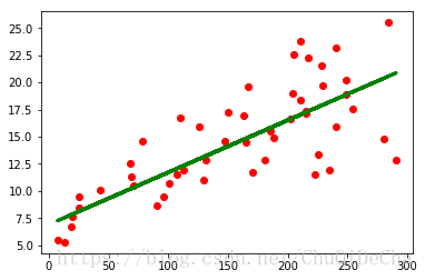
x = data[['TV']]
y = data['Sales']

# 划分训练集和测试集
x_train, x_test, y_train, y_test = train_test_split(x, y, random_state=1)

模型训练

# 模型训练
linreg = LinearRegression()
model = linreg.fit(x_train, y_train)

model

LinearRegression(copy_X=True, fit_intercept=True, n_jobs=1, normalize=False)

# 系数
model.coef_

array([0.04802945])

# 截距
linreg.intercept_

6.91197261886872

精度评定

y_hat = linreg.predict(np.array(x_test))

均方误差

$$MSE = \frac{1}{N}\sum^N(y-\hat{y})^2$$

mse = mean_squared_error(y_test, y_hat)
mse

10.310069587813155

$R^2$

• 样本总平方和TSS（Total Sum of Squares): $TSS = \sum(y_i-\overline{y})^2$
• 残差平方和RSS(Residual Sum of Squares): $TSS = \sum(y_i-\hat{y})^2$
• $R^2 = 1- \frac{RSS}{TSS}$
  
  • $R^2$越大，拟合效果越好
  • $R^2$最优值为1，若模型拟合效果较差，可能为负
  • 若预测值恒为样本均值，$R^2$ = 0

score = model.score(x_test,y_test)
score

0.5590828580007852

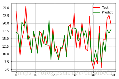
可视化结果

t = np.arange(len(x_test))
plt.plot(t, y_test, 'r-', linewidth=2, label='Test')
plt.plot(t, y_hat, 'g-', linewidth=2, label='Predict')
plt.legend(loc='upper right')
plt.grid()

plt.scatter(x_test, y_test,  color='red')
plt.plot(x_test, y_hat, color='green', linewidth=3)