Sklearn - SVM 支持向量机

---

相关官方文档：
https://scikit-learn.org/stable/modules/svm.html

---

一、训练一个线性分类器

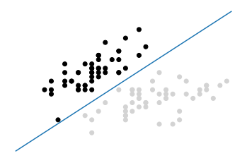
svc 试图找到一个能最大化分类之间间距的超平面

from sklearn.svm import LinearSVC
from sklearn import datasets
from sklearn.preprocessing import StandardScaler
import numpy as np 

iris = datasets.load_iris()  
iris_features = iris.data 
iris_target = iris.target 

# 以两个特征，两种分类 为例
# 原：3分类，4个特征
features = iris_features[:100, :2] 
target = iris_target[:100]  

target 

array([0, 0, 0, 0, 0, 0, 0, 0, 0, 0, 0, 0, 0, 0, 0, 0, 0, 0, 0, 0, 0, 0,
       0, 0, 0, 0, 0, 0, 0, 0, 0, 0, 0, 0, 0, 0, 0, 0, 0, 0, 0, 0, 0, 0,
       0, 0, 0, 0, 0, 0, 1, 1, 1, 1, 1, 1, 1, 1, 1, 1, 1, 1, 1, 1, 1, 1,
       1, 1, 1, 1, 1, 1, 1, 1, 1, 1, 1, 1, 1, 1, 1, 1, 1, 1, 1, 1, 1, 1,
       1, 1, 1, 1, 1, 1, 1, 1, 1, 1, 1, 1])

# iris_features
iris_target

array([0, 0, 0, 0, 0, 0, 0, 0, 0, 0, 0, 0, 0, 0, 0, 0, 0, 0, 0, 0, 0, 0,
       0, 0, 0, 0, 0, 0, 0, 0, 0, 0, 0, 0, 0, 0, 0, 0, 0, 0, 0, 0, 0, 0,
       0, 0, 0, 0, 0, 0, 1, 1, 1, 1, 1, 1, 1, 1, 1, 1, 1, 1, 1, 1, 1, 1,
       1, 1, 1, 1, 1, 1, 1, 1, 1, 1, 1, 1, 1, 1, 1, 1, 1, 1, 1, 1, 1, 1,
       1, 1, 1, 1, 1, 1, 1, 1, 1, 1, 1, 1, 2, 2, 2, 2, 2, 2, 2, 2, 2, 2,
       2, 2, 2, 2, 2, 2, 2, 2, 2, 2, 2, 2, 2, 2, 2, 2, 2, 2, 2, 2, 2, 2,
       2, 2, 2, 2, 2, 2, 2, 2, 2, 2, 2, 2, 2, 2, 2, 2, 2, 2]) 

---

# 标准化特征

scaler = StandardScaler()
features_standardized = scaler.fit_transform(features)  
# features_standardized

# 创建支持向量机 分类器
svc = LinearSVC(C=1.0)   
svc  # LinearSVC() 

# 训练模型
model = svc.fit(features_standardized, target)  
model # LinearSVC()

from matplotlib import pyplot as plt 

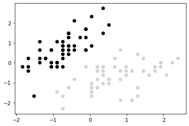
color = ['black' if c==0 else 'lightgray' for c in target ]
plt.scatter(features_standardized[:, 0], features_standardized[:, 1], c=color ) 

---

color = ['black' if c==0 else 'lightgray' for c in target ]
plt.scatter(features_standardized[:, 0], features_standardized[:, 1], c=color ) 

# 创建超平面

w = svc.coef_[0]
a = -w[0] /w[1] 
xx = np.linspace(-2.5, 2.5)
yy = a * xx - (svc.intercept_[0] ) / w[1] 

# 画出超平面 

plt.plot(xx, yy)

plt.axis('off')
plt.show() 

---

# w, a, xx, yy

# 创建一个新的样本点
new_ob = [[-2, 3]]

# 预测分类
svc.predict(new_ob) #  array([0])

---

二、使用核函数处理线性不可分的数据

from sklearn.svm import SVC

# 设置随机种子

np.random.seed(0)

# 生成两个特征
features = np.random.randn(200, 2)

# 使用异或门 创建线性不可分的数据
target_xor = np.logical_xor(features[:, 0] > 0, features[:, 1] > 0 ) 
target = np.where(target_xor, 0, 1)

# 创建一个有径向基核函数的支持向量机
svc = SVC(kernel='rbf', random_state=0, gamma=1, C=1) 

svc # SVC(C=1, gamma=1, random_state=0)

# 训练分类器
model = svc.fit(features, target) 

target_xor

array([False, False,  True,  True,  True, False, False, False,  True,
        True,  True,  True,  True,  True, False, False, False,  True,
       False, False, False,  True, False,  True, False,  True, False, 
        ...
       False, False,  True, False, False,  True,  True, False,  True,
        True,  True, False,  True, False, False,  True, False, False,
       False, False])

target 

array([1, 1, 0, 0, 0, 1, 1, 1, 0, 0, 0, 0, 0, 0, 1, 1, 1, 0, 1, 1, 1, 0,
       1, 0, 1, 0, 1, 0, 1, 1, 1, 1, 0, 0, 0, 1, 0, 0, 1, 0, 0, 0, 1, 0,
       ...
       0, 1, 1, 0, 1, 1, 0, 1, 1, 0, 0, 1, 0, 0, 0, 1, 0, 1, 1, 0, 1, 1,
       1, 1])

# 画出观察值和超平面决策边界 

from matplotlib.colors import ListedColormap

def plot_decision_regions(X, y, classifier):
    cmap = ListedColormap('red', 'blue')
    xx1, xx2 = np.meshgrid(np.arange(-3, 3, 0.02), np.arange(-3, 3, 0.02) )
    Z = classifier.predict(np.array([xx1.ravel(), xx2.ravel()]).T )
    Z = Z.reshape(xx1.shape)
    
    plt.contourf(xx1, xx2, Z, alpha=0.1, cmap=cmap) 
    
    for idx, cl in enumerate(np.unique(y)):
        plt.scatter(x=X[y==cl, 0], y=X[y==cl, 1],
                   alpha=0.8, c=cmap(idx), marker='+', label=cl  )

svc_linear = SVC(kernel='linear', random_state=0, C=1) 
svc_linear.fit(features, target) 

SVC(C=1, kernel='linear', random_state=0)

# 画出观察值 和 超平面
plot_decision_regions(features, target, classifier=svc_linear) 
plt.axis('off')
plt.show() 

# 创建一个使用径向基核函数的 SVC 
svc = SVC(kernel='rbf', random_state=0, gamma=1, C=1) 
model = svc.fit(features, target) 

plot_decision_regions(features, target, classifier=svc)  
plt.axis('off')
plt.show() 

使用 径向基核函数，可以创建一个分类效果 比 线性核函数好很多的 决策边界；

---

三、计算预测分类的概率

scaler = StandardScaler()
features_standardized = scaler.fit_transform(iris_features) 

svc = SVC(kernel='linear', probability=True, random_state=0)

model = svc.fit(features_standardized, iris_target)

# 创建一个新的观察值
new_ob = [[0.4, 0.4, 0.4, 0.4]]

# 查看观察值被预测为不同分类的概率 
model.predict_proba(new_ob) 

array([[0.00541761, 0.97348825, 0.02109414]])

---

四、识别支持向量

features = iris_features[:100, :]
target = iris_target[:100]

features_standardized = scaler.fit_transform(features)

svc = SVC(kernel='linear', random_state=0)
model = svc.fit(features_standardized, target) 

# 查看支持向量
model.support_vectors_ 

array([[-0.5810659 ,  0.42196824, -0.80497402, -0.50860702],
       [-1.52079513, -1.67737625, -1.08231219, -0.86427627],
       [-0.89430898, -1.4674418 ,  0.30437864,  0.38056609],
       [-0.5810659 , -1.25750735,  0.09637501,  0.55840072]])

# 查看支持向量，在观察中的索引值
model.support_ 

array([23, 41, 57, 98], dtype=int32)

# 查看每个分类有几个支持向量 
model.n_support_ 

array([2, 2], dtype=int32)

---

五、处理不均衡的分类

# 创建不均衡的观察值 
features = iris_features[40:100, :]
target = iris_target[40:100] 

# 创建目标向量，数值0 代表分类0，其他分类用 1 表示 
target = np.where((target==0), 0, 1) 
target 

array([0, 0, 0, 0, 0, 0, 0, 0, 0, 0, 1, 1, 1, 1, 1, 1, 1, 1, 1, 1, 1, 1,
       1, 1, 1, 1, 1, 1, 1, 1, 1, 1, 1, 1, 1, 1, 1, 1, 1, 1, 1, 1, 1, 1,
       1, 1, 1, 1, 1, 1, 1, 1, 1, 1, 1, 1, 1, 1, 1, 1])

features_standardized = scaler.fit_transform(features)

svc = SVC(kernel='linear', random_state=0, class_weight='balanced', C=1.0) 
model = svc.fit(features_standardized, target) 

---

2023-03-28