python_sklearn机器学习算法系列之SVM支持向量机算法

       本文主要目的是通过一段及其简单的小程序来快速学习python 中sklearn的svm 这一函数库的基本操作和使用，注意不是用python纯粹从头到尾自己构建svm ，既然sklearn提供了现成的我们直接拿来用就可以了，当然其原理十分重要，这里做简单介绍：

SVM方法是通过一个非线性映射p，把样本空间映射到一个高维乃至无穷维的特征空间中(Hilbert空间)，使得在原来的样本空间中非线性可分的问题转化为在特征空间中的线性可分的问题.简单地说，就是升维和线性化.升维，就是把样本向高维空间做映射，一般情况下这会增加计算的复杂性，甚至会引起"维数灾难"，因而人们很少问津.但是作为分类、回归等问题来说，很可能在低维样本空间无法线性处理的样本集，在高维特征空间中却可以通过一个线性超平面实现线性划分(或回归).一般的升维都会带来计算的复杂化，SVM方法巧妙地解决了这个难题:应用核函数的展开定理，就不需要知道非线性映射的显式表达式;由于是在高维特征空间中建立线性学习机，所以与线性模型相比，不但几乎不增加计算的复杂性，而且在某种程度上避免了"维数灾难".这一切要归功于核函数的展开和计算理论.

选择不同的核函数，可以生成不同的SVM，常用的核函数有以下4种:

⑴线性核函数K(x,y)=x·y;

⑵多项式核函数K(x,y)=[(x·y)+1]^d;

⑶径向基函数K(x,y)=exp(-|x-y|^2/d^2)

⑷二层神经网络核函数K(x,y)=tanh(a(x·y)+b).

更加详细的介绍建议看https://blog.csdn.net/lisi1129/article/details/70209945?locationNum=8&fps=1

svm既可以用来解决分类(SVC)又可以解决回归(SVR)下面将分别给出相关测试代码：

一   SVC:

在给出代码之前先简单介绍一个概念：核函数。其实质就是，在实际中，我们会经常遇到线性不可分的样例，此时，我们的常用做法是把样例特征映射到高维空间中去，但进一步，如果凡是遇到线性不可分的样例，一律映射到高维空间，那么这个维度大小是会高到可怕的。 此时，核函数就隆重登场了，核函数的价值在于它虽然也是讲特征进行从低维到高维的转换，但核函数绝就绝在它事先在低维上进行计算，而将实质上的分类效果表现在了高维上， 也就如上文所说的避免了直接在高维空间中的复杂计算(详细见https://blog.csdn.net/leonis_v/article/details/50688766)。SVM关键是选取核函数的类型，主要有线性内核，多项式内核，径向基内核（RBF），sigmoid核，至于怎样选取请看https://www.zhihu.com/question/21883548

在本次代码中支持向量分类(SVM_SVR)仅实验了线性内核和径向基内核（RBF）

代码：

#支持向量机分类
import numpy as np
import matplotlib as mpl
import matplotlib.pyplot as plt
import warnings
from sklearn import svm 
from sklearn import metrics
from sklearn import datasets
from sklearn.svm import SVC
from sklearn.model_selection import train_test_split

#忽略一些版本不兼容等警告
warnings.filterwarnings("ignore")

iris=datasets.load_iris()

x=iris.data[:,:2]                                                                        #为了后续的绘图方便只选取了前两个属性进行测试
y=iris.target
x_train, x_test, y_train, y_test = train_test_split(x, y, random_state=1, train_size=0.7)

#核心代码 gamma值越高越好，
clf1 = svm.SVC(C=0.8, kernel='rbf', gamma=10, decision_function_shape='ovr')            
clf2 = svm.SVC(C=0.8, kernel='linear',decision_function_shape='ovr')
clf3 = svm.SVC(C=0.8, kernel='rbf', gamma=20, decision_function_shape='ovr')
clf4 = svm.SVC(C=0.8, kernel='rbf', gamma=30, decision_function_shape='ovr')  
clf1.fit(x_train, y_train)
clf2.fit(x_train, y_train)
clf3.fit(x_train, y_train)
clf4.fit(x_train, y_train)

'''
#观察一些参数
y_predict=clf.predict(x_test)
print(clf.decision_function(x_test))                  #decision_function中每一列的值代表距离各类别的距离(正数代表该类，越大越属于该类，负数代表不属于该类)
print(clf.score(x_train, y_train))
print(metrics.classification_report(y_test,y_predict))
print(metrics.confusion_matrix(y_test,y_predict))

'''

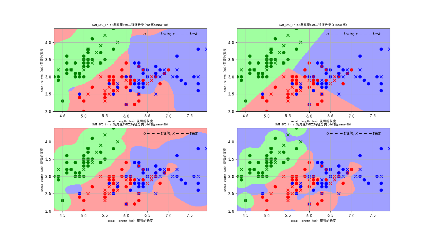
#绘图:图中形状为o的点是用来训练学习的学习集，图中形状为x的点为待预测的点
#根据形状为o的点来学习划分出图中区域(用pcolormesh画出),进而根据区域来预测x点，
#图中x点位置和表示类别颜色都是精确的，可以直观的看到预测误差
#注意:从图中来看有可能部分少量o点和x点重合，那是因为学习集合测试集有的数据非常相近
#类如（2.5,3.2）和（2.4,3.1）因为画布间隔问题，看上去就好好想挨着

#区域预测
x1_min, x1_max = x[:, 0].min(), x[:, 0].max()            # 第0列的范围
x2_min, x2_max = x[:, 1].min(), x[:, 1].max()            # 第1列的范围
x1, x2 = np.mgrid[x1_min:x1_max:200j, x2_min:x2_max:200j]# 生成网格采样点行列均为200点
area_smaple_point = np.stack((x1.flat, x2.flat), axis=1) # 将区域划分为一系列测试点去用学习的模型预测，进而根据预测结果画区域
area1_predict = clf1.predict(area_smaple_point)          # 所有区域点进行预测
area1_predict = area1_predict.reshape(x1.shape)          # 转化为和x1一样的数组因为用plt.pcolormesh(x1, x2, area_flag, cmap=classifier_area_color) 
                                                         # 时x1和x2组成的是200*200矩阵，area_flag要与它对应

area2_predict = clf2.predict(area_smaple_point)          
area2_predict = area2_predict.reshape(x1.shape)

area3_predict = clf3.predict(area_smaple_point)          
area3_predict = area3_predict.reshape(x1.shape)

area4_predict = clf4.predict(area_smaple_point)          
area4_predict = area4_predict.reshape(x1.shape)


mpl.rcParams['font.sans-serif'] = [u'SimHei']            #用来正常显示中文标签    
mpl.rcParams['axes.unicode_minus'] = False               #用来正常显示负号

classifier_area_color = mpl.colors.ListedColormap(['#A0FFA0', '#FFA0A0', '#A0A0FF'])  #区域颜色
cm_dark = mpl.colors.ListedColormap(['g', 'r', 'b'])#样本所属类别颜色


#第一个子图采用RBF核
plt.subplot(2,2,1)

plt.pcolormesh(x1, x2, area1_predict, cmap=classifier_area_color)                        
plt.scatter(x_train[:,0], x_train[:,1], c=y_train,marker='o', s=50, cmap=cm_dark)    
plt.scatter(x_test[:,0],x_test[:,1], c=y_test,marker='x', s=50, cmap=cm_dark)

plt.xlabel(iris.feature_names[0]+':花萼的长度', fontsize=8)  
plt.ylabel(iris.feature_names[1]+':花萼的宽度', fontsize=8)
plt.xlim(x1_min, x1_max)  
plt.ylim(x2_min, x2_max)
plt.title(u'SVM_SVC_iris:鸢尾花SVM二特征分类(rbf核gamma=10)', fontsize=8)
plt.text(x1_max-1.5, x1_min-0.1, u'$o---train ; x---test$')
plt.grid(True)


#第二个子图采用Linear核
plt.subplot(2,2,2)

plt.pcolormesh(x1, x2, area2_predict, cmap=classifier_area_color)                        
plt.scatter(x_train[:,0], x_train[:,1], c=y_train,marker='o', s=50, cmap=cm_dark)    
plt.scatter(x_test[:,0],x_test[:,1], c=y_test,marker='x', s=50, cmap=cm_dark)

plt.xlabel(iris.feature_names[0]+':花萼的长度', fontsize=8)  
plt.ylabel(iris.feature_names[1]+':花萼的宽度', fontsize=8)
plt.xlim(x1_min, x1_max)  
plt.ylim(x2_min, x2_max)
plt.title(u'SVM_SVC_iris:鸢尾花SVM二特征分类(linear核)', fontsize=8)
plt.text(x1_max-1.5, x1_min-0.1, u'$o---train ; x---test$')
plt.grid(True)

#第三个子图采用Linear核
plt.subplot(2,2,3)

plt.pcolormesh(x1, x2, area3_predict, cmap=classifier_area_color)                        
plt.scatter(x_train[:,0], x_train[:,1], c=y_train,marker='o', s=50, cmap=cm_dark)    
plt.scatter(x_test[:,0],x_test[:,1], c=y_test,marker='x', s=50, cmap=cm_dark)

plt.xlabel(iris.feature_names[0]+':花萼的长度', fontsize=8)  
plt.ylabel(iris.feature_names[1]+':花萼的宽度', fontsize=8)
plt.xlim(x1_min, x1_max)  
plt.ylim(x2_min, x2_max)
plt.title(u'SVM_SVC_iris:鸢尾花SVM二特征分类(rbf核gamma=20)', fontsize=8)
plt.text(x1_max-1.5, x1_min-0.1, u'$o---train ; x---test$')
plt.grid(True)

#第四个子图采用Linear核
plt.subplot(2,2,4)

plt.pcolormesh(x1, x2, area4_predict, cmap=classifier_area_color)                        
plt.scatter(x_train[:,0], x_train[:,1], c=y_train,marker='o', s=50, cmap=cm_dark)    
plt.scatter(x_test[:,0],x_test[:,1], c=y_test,marker='x', s=50, cmap=cm_dark)

plt.xlabel(iris.feature_names[0]+':花萼的长度', fontsize=8)  
plt.ylabel(iris.feature_names[1]+':花萼的宽度', fontsize=8)
plt.xlim(x1_min, x1_max)  
plt.ylim(x2_min, x2_max)
plt.title(u'SVM_SVC_iris:鸢尾花SVM二特征分类(rbf核gamma=30)', fontsize=8)
plt.text(x1_max-1.5, x1_min-0.1, u'$o---train ; x---test$')
plt.grid(True)


plt.show()

运行结果：

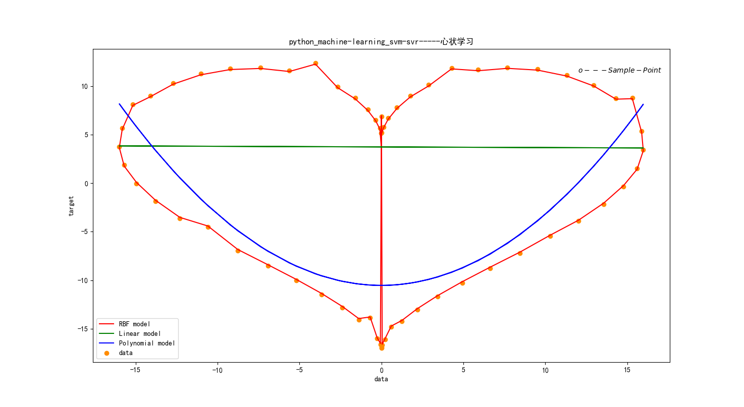
   二 SVR:

   代码：

#SVM回归
import matplotlib as mpl
import numpy as np
import warnings
from sklearn.svm import SVR  
import matplotlib.pyplot as plt

#忽略一些版本不兼容等警告
warnings.filterwarnings("ignore")

#产生心状坐标
t = np.arange(0,2*np.pi,0.1)
x = 16*np.sin(t)**3
x=x[:, np.newaxis]
y = 13*np.cos(t)-5*np.cos(2*t)-2*np.cos(3*t)-np.cos(4*t)
y[::7]+= 2* (1 - np.random.rand(9))                     #增加噪声，在每数2个数的时候增加一点噪声



svr_rbf=SVR(kernel='rbf', C=1e3, gamma=200)      
svr_lin = SVR(kernel='linear', C=1500)  
svr_poly = SVR(kernel='poly', C=1500, degree=2)

#三种核函数预测
y_rbf = svr_rbf.fit(x,y).predict(x)
y_lin = svr_lin.fit(x,y).predict(x)
y_poly = svr_poly.fit(x,y).predict(x)

#为了后面plt.text定位
x1_min, x1_max = x[:].min(), x[:].max()          
x2_min, x2_max = y[:].min(), y[:].max()


mpl.rcParams['font.sans-serif'] = [u'SimHei']            #用来正常显示中文标签    
mpl.rcParams['axes.unicode_minus'] = False

plt.scatter(x, y, color='darkorange', label='data')  
plt.hold('on')

plt.plot(x, y_rbf, color='r',  label='RBF model')  
plt.plot(x, y_lin, color='g',  label='Linear model')  
plt.plot(x, y_poly, color='b', label='Polynomial model')

plt.xlabel('data')  
plt.ylabel('target')  
plt.title('python_machine-learning_svm-svr-----心状学习')  
plt.legend()
plt.text(x1_max-4, x2_max-1, u'$o---Sample-Point$')
plt.show()

运行结果：

更多算法可以参看博主其他文章，或者github：https://github.com/Mryangkaitong/python-Machine-learning