SVM支持向量机

支持向量机SVM（Support Vector Machine）

【关键词】支持向量，最大几何间隔，拉格朗日乘子法

一、支持向量机的原理

Support Vector Machine。支持向量机，其含义是通过支持向量运算的分类器。其中“机”的意思是机器，可以理解为分类器。
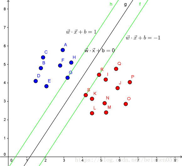
那么什么是支持向量呢？在求解的过程中，会发现只根据部分数据就可以确定分类器，这些数据称为支持向量。
见下图，在一个二维环境中，其中点R，S，G点和其它靠近中间黑线的点可以看作为支持向量，它们可以决定分类器，也就是黑线的具体参数。

解决的问题：

• 线性分类

在训练数据中，每个数据都有n个的属性和一个二类类别标志，我们可以认为这些数据在一个n维空间里。我们的目标是找到一个n-1维的超平面（hyperplane），这个超平面可以将数据分成两部分，每部分数据都属于同一个类别。
其实这样的超平面有很多，我们要找到一个最佳的。因此，增加一个约束条件：这个超平面到每边最近数据点的距离是最大的。也成为最大间隔超平面（maximum-margin hyperplane）。这个分类器也成为最大间隔分类器（maximum-margin classifier）。
支持向量机是一个二类分类器。

• 非线性分类

SVM的一个优势是支持非线性分类。它结合使用拉格朗日乘子法和KKT条件，以及核函数可以产生非线性分类器。

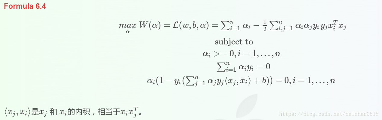
SVM的目的是要找到一个线性分类的最佳超平面 f(x)=xw+b=0。求 w 和 b。

首先通过两个分类的最近点，找到f(x)的约束条件。

有了约束条件，就可以通过拉格朗日乘子法和KKT条件来求解，这时，问题变成了求拉格朗日乘子αi 和 b。

对于异常点的情况，加入松弛变量ξ来处理。

非线性分类的问题：映射到高维度、使用核函数。

线性分类及其约束条件

SVM的解决问题的思路是找到离超平面的最近点，通过其约束条件求出最优解。

最大几何间隔（geometrical margin）

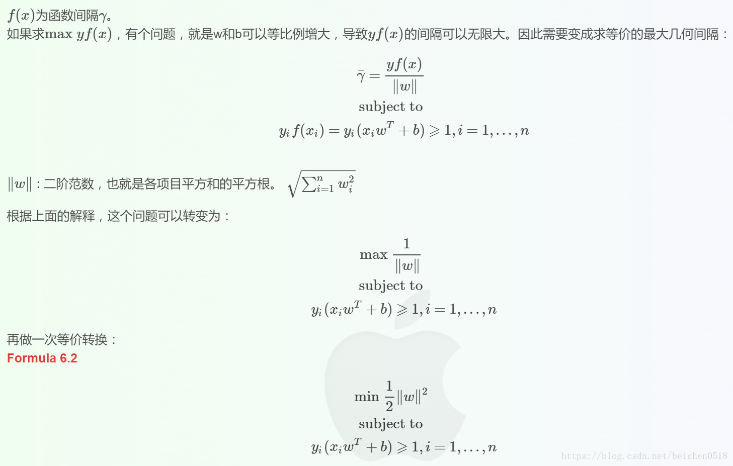
求解问题w,b

我们使用拉格朗日乘子法(http://blog.csdn.net/on2way/article/details/47729419)
来求w和b，一个重要原因是使用拉格朗日乘子法后,还可以解决非线性划分问题。
拉格朗日乘子法可以解决下面这个问题：

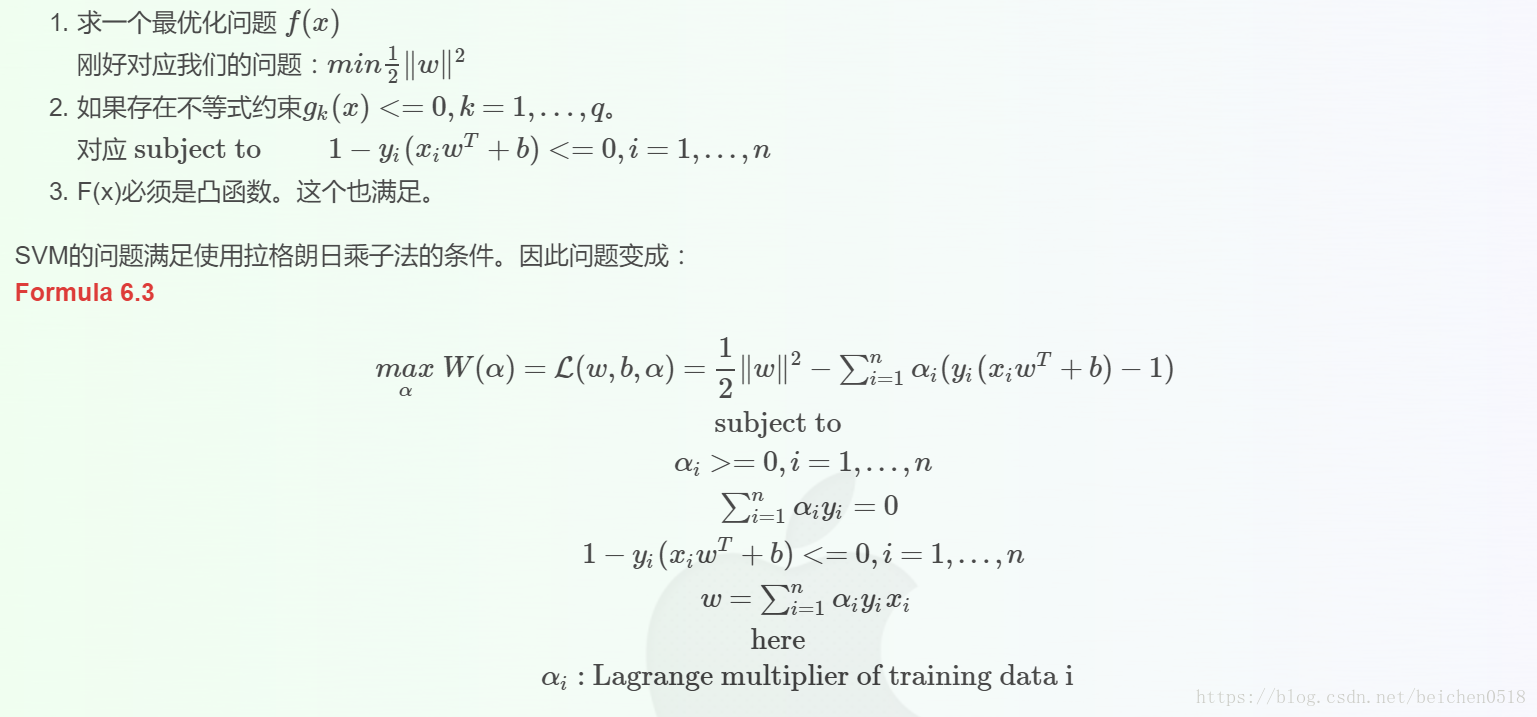
消除w之后变为：

可见使用拉格朗日乘子法后，求w,b的问题变成了求拉格朗日乘子αi和b的问题。
到后面更有趣，变成了不求w了，因为αi可以直接使用到分类器中去，并且可以使用αi支持非线性的情况.

二、实战

1、画出决策边界

导包sklearn.svm

# SVC用于分类
from sklearn.svm import SVC

import numpy as np

import matplotlib.pyplot as plt

随机生成数据，并且进行训练np.r_[]

#画二维的点，特征只有两个
# 两簇点
dot1 = np.random.randn(20, 2) - [2, 2]
dot2 = np.random.randn(20, 2) + [3, 2]

# 将两簇点行级联
dot = np.concatenate([dot1, dot2])
dot.shape

• 输出

  (40, 2)

# 两类点分类

target = [0] * 20 + [-1] * 20

训练模型，并训练

# It must be one of 'linear', 'poly', 'rbf', 'sigmoid', 'precomputed' or a callable.
# kernel 核心 linear 线性 poly 多项式 rbf基于半径的    
svc = SVC(kernel= 'linear')

X_train = dot
y_train = target

svc.fit(X_train, y_train)

• 输出

  SVC(C=1.0, cache_size=200, class_weight=None, coef0=0.0,
  decision_function_shape=’ovr’, degree=3, gamma=’auto’, kernel=’linear’,
  max_iter=-1, probability=False, random_state=None, shrinking=True,
  tol=0.001, verbose=False)

提取系数获取斜率

X_train.shape

• 输出

  (40, 2)

coef_ = svc.coef_

线性方程的截距

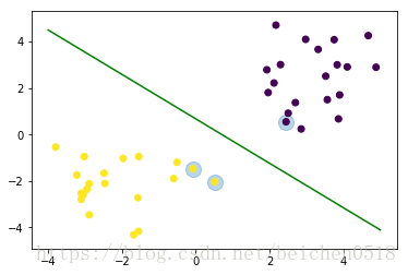
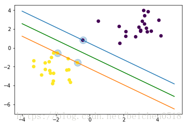
b = svc.intercept_

# f（x, y） = w1 * x + w2 * y + b

# 支持 向量 一般是3个 有的时候是两个

support_vectors_ = svc.support_vectors_
support_vectors_ 

• 输出

  array([[ 2.4481023 , 0.54268437],
  [ 0.51456029, -2.03510616],
  [-0.0747407 , -1.47089428]])

# 把支持向量的点给找出来
plt.scatter(support_vectors_[:,0], support_vectors_[:,1], s=200, alpha=0.3)
plt.scatter(dot[:,0], dot[:,1], c=target)

<matplotlib.collections.PathCollection at 0x12864e48>

# 3 维度的图形
from mpl_toolkits.mplot3d import Axes3D

X_train() 40, 2
2 个属性 0 代表x 1 代表y

coef[0,0]代表w1
coef[0,1]代表w2
b截距

三维降二维
f(x,y) = w1 * x + w2 * y + b
0 = w1 * x + w2 * y + b
y = -coef_[0,0]/coef_[0,1] * x - b /coef_[0,1]

# 二维中的分类线
# y = wx + b
w = -coef_[0,0]/coef_[0,1]
b_ = - b /coef_[0,1]

# 线生成一个范围
x = np.linspace(-4, 5, 100)

y = w * x + b_

# 画一个分类线
plt.plot(x, y, c='g')
plt.scatter(support_vectors_[:,0], support_vectors_[:,1], s=200, alpha=0.3)
plt.scatter(dot[:,0], dot[:,1], c=target)

<matplotlib.collections.PathCollection at 0x128c00b8>

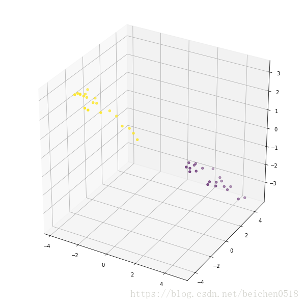
# x, y, z
# f(x, y) = w1 * x + w2 * y +b

x1 = dot[:,0]
y1 = dot[:,1]
w1 = coef_[0,0]
w2 = coef_[0,1]
z1 = w1 * x1 + w2 * y1 + b

fig = plt.figure(figsize=(8, 8))
axes3D = Axes3D(fig)
axes3D.scatter(x1, y1, z1,c=y_train)

<mpl_toolkits.mplot3d.art3d.Path3DCollection at 0xc44f9e8>

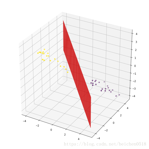
a1, b1 = np.meshgrid(x, y)
z2 = w1 * a1 + w2 * b1 + b
fig = plt.figure(figsize=(8, 8))
axes3D = Axes3D(fig)
axes3D.scatter(x1, y1, z1,c=y_train)
axes3D.plot_surface(x, y, z2, color='red')

<mpl_toolkits.mplot3d.art3d.Poly3DCollection at 0x1336d7b8>

a1

array([[-4.        , -3.90909091, -3.81818182, ...,  4.81818182,
         4.90909091,  5.        ],
       [-4.        , -3.90909091, -3.81818182, ...,  4.81818182,
         4.90909091,  5.        ],
       [-4.        , -3.90909091, -3.81818182, ...,  4.81818182,
         4.90909091,  5.        ],
       ...,
       [-4.        , -3.90909091, -3.81818182, ...,  4.81818182,
         4.90909091,  5.        ],
       [-4.        , -3.90909091, -3.81818182, ...,  4.81818182,
         4.90909091,  5.        ],
       [-4.        , -3.90909091, -3.81818182, ...,  4.81818182,
         4.90909091,  5.        ]])

上边界和下边界

support_vectors_

# 需要支持的三点
support_vectors_

• 输出

  array([[-0.4115882 , 0.81065679],
  [-1.91821725, -0.55639636],
  [-0.73355567, -1.57297753]])

# 上面的一个点先取出来
vector_up = support_vectors_[0]
vector_down = support_vectors_[-1]

绘制图形

# 上面的点
y_up = w * x + vector_up[1] - w * vector_up[0]
y_down = w * x + vector_down[1] - w * vector_down[0]
plt.scatter(support_vectors_[:,0], support_vectors_[:,1], s=200, alpha=0.3)
plt.scatter(dot[:,0], dot[:,1], c=target)
plt.plot(x, y_up, x, y_down)
plt.plot(x, y, c='g')

[<matplotlib.lines.Line2D at 0xca79cf8>]

2、SVM分离坐标点

导包

# 基于半径的内核 kernel='rbf'
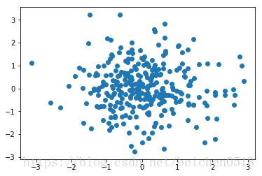
svc = SVC(kernel='rbf')

创造-3到3范围的点以及meshgrid

data = np.random.randn(300,2)
plt.scatter(data[:,0], data[:,1])

<matplotlib.collections.PathCollection at 0x13363630>

创造模型：rbf，训练数据

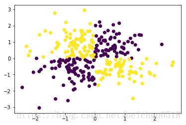
# xor 异或 假如值是一个序列 ，用每个序列中相同的下标做对比
# 第一象限和第三象限 x轴y轴符号相同
# 第二象限和第四象限 x轴y轴符号相异
np.logical_xor([1,0],[1,0])

• 输出

  array([False, False])

target = np.logical_xor(data[:,0]>0, data[:,1]>0)

# target
# 让第一象限和第三象限是一类，让第二象限和第四象限是一类

plt.scatter(data[:,0], data[:,1], c=target)

<matplotlib.collections.PathCollection at 0x134adda0>

X_train = data
y_train = target

svc.fit(X_train,y_train)

• 输出

  SVC(C=1.0, cache_size=200, class_weight=None, coef0=0.0,
  decision_function_shape=’ovr’, degree=3, gamma=’auto’, kernel=’rbf’,
  max_iter=-1, probability=False, random_state=None, shrinking=True,
  tol=0.001, verbose=False)

# 缺的多个点
x_x = np.linspace(-3.3, 3, 500)
y_y = np.linspace(-3.3, 3.3, 500)

# 网格线
xx, yy = np.meshgrid(x_x, y_y)
# np.c 将x轴和y轴融合成点
# ravel 展开 也就是降成一维的数组
xy = np.c_[xx.ravel(), yy.ravel()]

svc.predict(xy)

• 输出

  array([False, False, False, …, False, False, False])

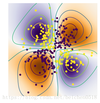
# 样本X超平面的距离
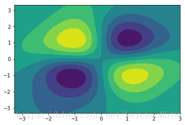
z = svc.decision_function(xy)

绘制图形
绘制测试点到分离超平面的距离(decision_function)
绘制轮廓线
绘制训练点

# imshow 画图的数据是二维的
# extent 选取轴的范围， 它的值是一个序列， 必须成对出现
plt.figure(figsize=(6,6))
plt.imshow(z.reshape(500, 500), extent=[-3.3, 3,-3.3, 3.3], cmap=plt.cm.PuOr_r)
plt.scatter(data[:,0], data[:,1], c=target)

# contour 是一个三维的绘制 轮廓线
plt.contour(xx,yy, z.reshape(500, 500))
plt.axis('off')

• 输出

  (-3.3, 3.0, -3.3, 3.3)

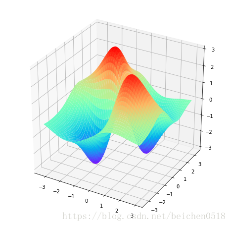
# 是一个三维的绘制 轮廓面
plt.contourf(xx,yy, z.reshape(500, 500))

<matplotlib.contour.QuadContourSet at 0x10368a20>

# 画个3d图
plt.figure(figsize=(8,8))
axes3d = plt.subplot(projection='3d')
axes3d.plot_surface(xx,yy,z.reshape(500,500),cmap='rainbow')

<mpl_toolkits.mplot3d.art3d.Poly3DCollection at 0x12f93d68>

3、使用多种核函数对iris数据集进行分类

导包

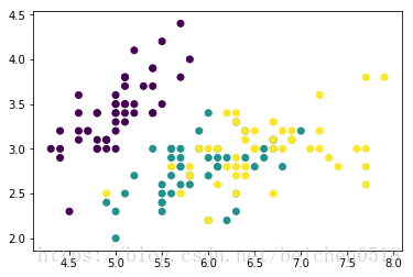
import sklearn.datasets as datasets

iris = datasets.load_iris()
# 鸢尾花有四个属性，也就是四个维度

提取数据只提取两个特征，方便画图
创建支持向量机的模型：’linear’, ‘poly’(多项式), ‘rbf’(Radial Basis Function:基于半径函数),

X_train = iris['data'][:,:2]
y_train = iris['target']

svc_linear = SVC(kernel='linear')
svc_poly = SVC(kernel='poly')
svc_rbf = SVC(kernel='rbf') 

训练模型

svc_linear.fit(X_train,y_train)
svc_poly.fit(X_train,y_train)
svc_rbf.fit(X_train,y_train)

• 输出

  SVC(C=1.0, cache_size=200, class_weight=None, coef0=0.0,
  decision_function_shape=’ovr’, degree=3, gamma=’auto’, kernel=’rbf’,
  max_iter=-1, probability=False, random_state=None, shrinking=True,
  tol=0.001, verbose=False)

图片背景点

plt.scatter(X_train[:,0],X_train[:,1],c=y_train)

<matplotlib.collections.PathCollection at 0x111cecc0>

xx, yy = np.meshgrid(np.linspace(4, 8, 300), np.linspace(1.9,4.5,300))

xy = np.c_[xx.ravel(),yy.ravel()]

# 预测
linear_y_ = svc_linear.predict(xy)
poly_y_ = svc_poly.predict(xy)
rbf_y_ = svc_rbf.predict(xy)

# 绘制图形

plt.figure(figsize=(12,10))
axes = plt.subplot(2,2,1)
axes.contourf(xx, yy, linear_y_.reshape(300, 300), cmap='cool')
axes.scatter(X_train[:,0],X_train[:,1],c=y_train, cmap='gray')
# axes.scatter(xx.ravel(), yy.ravel(), c = linear_y_)

axes = plt.subplot(2,2,2)
axes.contourf(xx, yy, poly_y_.reshape(300, 300), cmap='cool')
axes.scatter(X_train[:,0],X_train[:,1],c=y_train, cmap='gray')

axes = plt.subplot(2,2,3)
axes.contourf(xx, yy, rbf_y_.reshape(300, 300), cmap='cool')
axes.scatter(X_train[:,0],X_train[:,1],c=y_train, cmap='gray')

<matplotlib.collections.PathCollection at 0x16f77da0>

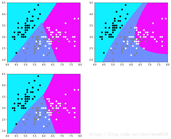
svc_linear.score(X_train,y_train)

• 输出

  0.82

svc_poly.score(X_train,y_train)

• 输出

  0.8133333333333334

svc_rbf.score(X_train,y_train)

• 输出

  0.8266666666666667

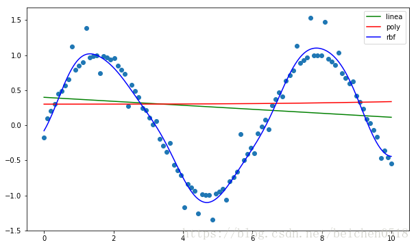
4、使用SVM多种核函数进行回归

导包

from sklearn.svm import SVR

自定义样本点rand，并且生成sin值

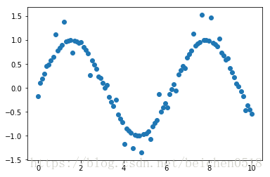
# 生成一个正弦波
X_train = np.linspace(0, 10, 100).reshape(-1,1)

y_train = np.sin(X_train)

数据加噪

y_train[::4] += np.random.randn(25,1) * 0.3

plt.scatter(X_train, y_train)

<matplotlib.collections.PathCollection at 0x16547080>

# target都是一维的值
y_train.ravel().shape

• 输出

  (100,)

建立模型，训练数据，并预测数据，预测训练数据就行

svr_linear = SVR(kernel='linear')
svr_poly = SVR(kernel='poly')
svr_rbf = SVR(kernel='rbf')

svr_linear.fit(X_train, y_train)
svr_poly.fit(X_train, y_train)
svr_rbf.fit(X_train, y_train)

• 输出

  SVR(C=1.0, cache_size=200, coef0=0.0, degree=3, epsilon=0.1, gamma=’auto’,
  kernel=’rbf’, max_iter=-1, shrinking=True, tol=0.001, verbose=False)

# 预测数据
X_test = np.linspace(0, 10, 1000).reshape(-1,1)

linear_y_ = svr_linear.predict(X_test)
poly_y_ = svr_poly.predict(X_test)
rbf_y_ = svr_rbf.predict(X_test)

绘制图形，观察三种支持向量机内核不同

plt.figure(figsize=(10,6))
plt.scatter(X_train, y_train)
plt.plot(X_test, linear_y_, c='g', label='linea')
plt.plot(X_test, poly_y_, c='r', label='poly')
plt.plot(X_test, rbf_y_, c='b', label='rbf')
plt.legend()

<matplotlib.legend.Legend at 0x19b76c50>