传统机器学习(七)支持向量机(2)sklearn中的svm

传统机器学习(七)支持向量机(2)sklearn中的svm

2 sklearn中的svm

2.1 LinearSVC及SVC参数详解

2.1.1 SVC参数

class sklearn.svm.SVC(*,
                      C=1.0, 
                      kernel='rbf', 
                      degree=3, 
                      gamma='scale', 
                      coef0=0.0, 
                      shrinking=True, 
                      probability=False, 
                      tol=0.001, 
                      cache_size=200, 
                      class_weight=None, 
                      verbose=False, 
                      max_iter=-1, 
                      decision_function_shape='ovr', 
                      break_ties=False, 
                      random_state=None
                     )

用于分类，用libsvm实现，参数如下：

• C : 惩罚项，默认为1.0，C越大容错空间越小；C越小，容错空间越大
• kernel : 核函数的类型，可选参数为：
  • “linear” : 线性核函数
  • “poly” : 多项式核函数
  • “rbf” : 高斯核函数(默认)
  • “sigmod” : sigmod核函数
  • “precomputed” : 核矩阵，表示自己提前计算好核函数矩阵
• degree : 多项式核函数的阶，默认为3，只对多项式核函数生效
• gamma : 核函数系数，可选，float类型，默认为auto。只对’rbf’ ,’poly’ ,’sigmod’有效。如果gamma为auto，代表其值为样本特征数的倒数，即1/n_features
• coef0 ：核函数中的独立项，float类型，可选，默认为0.0。只有对’poly’ 和,’sigmod’核函数有用，是指其中的参数c
• probability : 是否启用概率估计，bool类型，可选参数，默认为False，这必须在调用fit()之前启用，并且会fit()方法速度变慢
• tol ：svm停止训练的误差精度，float类型，可选参数，默认为1e^-3
• cache_size ：内存大小，float，可选，默认200。指定训练所需要的内存，单位MB
• class_weight：类别权重，dict类型或str类型，可选，默认None。给每个类别分别设置不同的惩罚参数C，如果没有，则会给所有类别都给C=1，即前面指出的C。如果给定参数’balance’，则使用y的值自动调整与输入数据中的类频率成反比的权重
• max_iter：最大迭代次数，int类型，默认为-1，不限制
• decision_function_shape ：决策函数类型，可选参数’ovo’和’ovr’，默认为’ovr’。’ovo’表示one vs one，’ovr’表示one vs rest。（多分类）
• random_state ：数据洗牌时的种子值，int类型，可选，默认为None

2.1.2 LinearSVC参数

class sklearn.svm.LinearSVC(
    penalty='l2', 
    loss='squared_hinge', 
    *, 
    dual=True, 
    tol=0.0001, 
    C=1.0, 
    multi_class='ovr', 
    fit_intercept=True, 
    intercept_scaling=1, 
    class_weight=None, 
    verbose=0, 
    random_state=None, 
    max_iter=1000
)

LinearSVC（Linear Support Vector Classification）线性支持向量机，核函数是 linear，不是基于libsvm实现的
参数：

• C：目标函数的惩罚系数C，默认C = 1.0；
• loss：指定损失函数. squared_hinge(默认), squared_hinge
• penalty ： 惩罚方式，str类型，l1, l2
• dual ：选择算法来解决对偶或原始优化问题。当nsamples>nfeatures时dual=false
• tol ：svm结束标准的精度， 默认是 1e - 3
• multi_class：如果y输出类别包含多类，用来确定多类策略， ovr表示一对多，“crammer_singer”优化所有类别的一个共同的目标 。如果选择“crammer_singer”，损失、惩罚和优化将会被被忽略。
• max_iter : 要运行的最大迭代次数。int，默认1000

2.2 LinearSVC及SVC使用案例

2.2.1 鸢尾花数据集在线性SVM上的应用

线性SVM有两种方式实现：

• LinearSVC(C=1)
• SVC(C=1, kernel="linear")

import numpy as np
import os
%matplotlib inline
import matplotlib
import matplotlib.pyplot as plt
plt.rcParams['axes.labelsize'] = 14
plt.rcParams['xtick.labelsize'] = 12
plt.rcParams['ytick.labelsize'] = 12
import warnings
warnings.filterwarnings('ignore')


from sklearn.svm import SVC
from sklearn.datasets import load_iris

# 选择鸢尾花数据集的两列，方便画图
iris = load_iris()
X = iris['data'][:, (2,3)]
y = iris['target']

# 只选择两个种类的鸢尾花数据
setosa_versi = (y == 0) | (y == 1)
X = X[setosa_versi]
y = y[setosa_versi]


# 训练，常数C越大，容错空间越小，上下支持面之间的距离越小；常数C越小，容错空间越大，上下支持面之间的距离越大
svm_clf = SVC(kernel='linear',C=100000000)
svm_clf.fit(X,y)

# 绘制决策边界
def plot_svc_decision_boundary(svm_clf,xmin,xmax,sv=True):
    # linearsvc.coef_是所有特征的权重
    w = svm_clf.coef_[0]
    # linearsvc.intercept_是截距
    b = svm_clf.intercept_[0]
    
    x0 = np.linspace(xmin, xmax, 200)
    # 决策边界方程为：w[0]x0 + w[1]x1 = 0
    # 这里计算x1的值
    decision_boundary = - w[0]/w[1] * x0 - b/w[1]
    # 支持面距离判别面之间的距离margin
    margin = 1 / w[1]
    # 上支持面，在这里是x1 + margin
    gutter_up = decision_boundary + margin
    # 下支持面，在这里是x1 - margin
    gutter_dw = decision_boundary - margin
    
    # 是否画出支持向量
    if sv:
        svs = svm_clf.support_vectors_  # 支持向量
        plt.scatter(svs[:,0],svs[:,1],s=180)
    plt.plot(x0,decision_boundary,'k-',linewidth=2)
    plt.plot(x0,gutter_up,'k--',linewidth=2)
    plt.plot(x0,gutter_dw,'k--',linewidth=2)

plt.figure(figsize=(12,8))
plot_svc_decision_boundary(svm_clf,0,5.5)
plt.plot(X[:,0][y==1],X[:,1][y==1],'bs')
plt.plot(X[:,0][y==0],X[:,1][y==0],'yo')
plt.axis([0,5.5,0,2])
plt.show()

# 在这里把C值调小一些，我们可以看到容错空间越大，上下支持面之间的距离越大
# 此时的支撑向量：指的是落在支持面上的样本，及支持面没支持住的样本
svm_clf_2 = SVC(kernel='linear',C=0.01)
svm_clf_2.fit(X,y)


plt.figure(figsize=(12,8))
plot_svc_decision_boundary(svm_clf_2,0,5.5)
plt.plot(X[:,0][y==1],X[:,1][y==1],'bs')
plt.plot(X[:,0][y==0],X[:,1][y==0],'yo')
plt.axis([0,5.5,0,2])
plt.show()

2.2.2 多项式核函数

这里可以手动使用 PolynomialFeature将数据升维，再用LinearSVC进行分类。也可以直接使用SVC指定多项式核函数，即：

1、用LinearSVC，需要用PolynomialFeatures升维

from sklearn.datasets import make_moons

# 使用sklearn自带的moon数据
X, y = make_moons(n_samples=100,noise=0.15,random_state=42)

def plot_dataset(X,y,axis):
    plt.plot(X[:,0][y == 0],X[:,1][y == 0],'bs')
    plt.plot(X[:,0][y == 1],X[:,1][y == 1],'go')
    plt.axis(axis)
    plt.grid(True,which='both')


plot_dataset(X,y,[-1.5,2.5,-1,1.5])
plt.show()

from sklearn.preprocessing import PolynomialFeatures

# 使用LinearSVC分类，使用pipeline封装一下
poly_pipeline = Pipeline(steps=[
    ("ploy_features",PolynomialFeatures(degree=3)),
    ("scaler",StandardScaler()),
    ("svm_clf",LinearSVC(C=10,loss='hinge'))
])

poly_pipeline.fit(X,y)

# 画出决策边界
def plot_pred(clf,axes):
    x0s = np.linspace(axes[0],axes[1],100)
    x1s = np.linspace(axes[2],axes[3],100)
    x0,x1 = np.meshgrid(x0s,x1s)
    # x0 和 x1 被拉成一列，然后拼接成10000行2列的矩阵，表示所有点
    X = np.c_[x0.ravel(),x1.ravel()]
    # 二维点集才可以用来预测
    y_pred = clf.predict(X).reshape(x0.shape)
    # 等高线
    plt.contourf(x0,x1,y_pred,alpha=0.2)

plot_pred(poly_pipeline,[-1.5,2.5,-1,1.5])
plot_dataset(X,y,[-1.5,2.5,-1,1.5])
plt.show()

2、用SVC() 指定kernel=poly

ploy_kernel_svm_clf1 = Pipeline(
    steps=[
        ("scaler",StandardScaler()),
        ("svm_clf",SVC(kernel='poly',degree=3,coef0=1,C=5))
    ]
)

ploy_kernel_svm_clf1.fit(X,y)


# 可以看到degree越大，分类效果越好，但是也容易造成模型过拟合、模型复杂度提高
ploy_kernel_svm_clf2 = Pipeline(
    steps=[
        ("scaler",StandardScaler()),
        ("svm_clf",SVC(kernel='poly',degree=10,coef0=100,C=5))
    ]
)

ploy_kernel_svm_clf2.fit(X,y)

plt.figure(figsize=(12,5))
plt.subplot(121)
plot_pred(ploy_kernel_svm_clf1,[-1.5,2.5,-1,1.5])
plot_dataset(X,y,[-1.5,2.5,-1,1.5])

plt.subplot(122)
plot_pred(ploy_kernel_svm_clf2,[-1.5,2.5,-1,1.5])
plot_dataset(X,y,[-1.5,2.5,-1,1.5])
plt.show()

2.2.3 高斯核函数

gamma1,gamma2 = 0.1,5
C1,C2 = 0.001,1000

params = (gamma1,C1),(gamma1,C2),(gamma2,C1),(gamma2,C2)

svm_clfs = []

for gamma,C in params:
    rbf_pipeline = Pipeline(
        steps=[
             ("scaler",StandardScaler()),
             ("svm_clf",SVC(kernel='rbf',gamma=gamma,C=C))
        ]
    )
    rbf_pipeline.fit(X,y)
    svm_clfs.append(rbf_pipeline)

plt.figure(figsize=(11,7))
for  i,svm_clf in enumerate(svm_clfs):
    plt.subplot(221+i)
    plot_pred(svm_clf,[-1.5,2.5,-1,1.5])
    plot_dataset(X,y,[-1.5,2.5,-1,1.5])
    gamma,C = params[i]
    plt.title("gamma = {},C = {}".format(gamma,C))

plt.show()

• gamma参数越大，高斯分布越窄

• 常数C越大，容错空间越小

2.3 SVM应用于图像识别案例

我们将尝试做的是，给出一个人脸的图像，预测它可能属于列表中的哪些人。

学习集将是一组人脸的带标记图像，我们将尝试学习一种模型，可以预测没见过的实例的标签。
第一种直观的方法是将图像像素用作学习算法的特征，因此像素值将是我们的学习属性，而个体的标签将是我们的目标类。

1、数据探索

import numpy as np
import matplotlib.pyplot as plt
from sklearn.datasets import fetch_olivetti_faces

%matplotlib inline
plt.rcParams['axes.labelsize'] = 14
plt.rcParams['xtick.labelsize'] = 12
plt.rcParams['ytick.labelsize'] = 12
import warnings
warnings.filterwarnings('ignore')


'''
该数据集包含 40 个不同人脸的400张灰度的64*64像素的人脸图像。
拍摄的照片采用不同的光线条件和面部表情（包括睁眼/闭眼，微笑/不笑，戴眼镜/不戴眼镜）

提供一个百度网盘的连接，可以手动下载
链接： https://pan.baidu.com/s/1ofeOk6hE4tMA-AYPJzW7cg
提取码：1111

将人脸图像数据集olivetti_py3.pkz放入到data目录下
'''

faces = fetch_olivetti_faces(data_home='./data/')
# 打印数据集信息
print(faces.DESCR)

.. _olivetti_faces_dataset:

The Olivetti faces dataset
--------------------------

`This dataset contains a set of face images`_ taken between April 1992 and 
April 1994 at AT&T Laboratories Cambridge. The
:func:`sklearn.datasets.fetch_olivetti_faces` function is the data
fetching / caching function that downloads the data
archive from AT&T.

.. _This dataset contains a set of face images: https://cam-orl.co.uk/facedatabase.html

As described on the original website:

    There are ten different images of each of 40 distinct subjects. For some
    subjects, the images were taken at different times, varying the lighting,
    facial expressions (open / closed eyes, smiling / not smiling) and facial
    details (glasses / no glasses). All the images were taken against a dark
    homogeneous background with the subjects in an upright, frontal position 
    (with tolerance for some side movement).

**Data Set Characteristics:**

    =================   =====================
    Classes                                40
    Samples total                         400
    Dimensionality                       4096
    Features            real, between 0 and 1
    =================   =====================

The image is quantized to 256 grey levels and stored as unsigned 8-bit 
integers; the loader will convert these to floating point values on the 
interval [0, 1], which are easier to work with for many algorithms.

The "target" for this database is an integer from 0 to 39 indicating the
identity of the person pictured; however, with only 10 examples per class, this
relatively small dataset is more interesting from an unsupervised or
semi-supervised perspective.

The original dataset consisted of 92 x 112, while the version available here
consists of 64x64 images.

When using these images, please give credit to AT&T Laboratories Cambridge.

​

'''
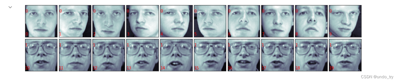
查看faces对象的内容，我们得到以下属性：images，data和target。
images包含表示为64 x 64像素矩阵的 400 个图像。
data包含相同的 400 个图像，但是作为 4096 个像素的数组。
target是一个具有目标类的数组，范围从 0 到 39。
'''

print(faces.keys())
print(faces.images.shape)
print(faces.data.shape)
print(faces.target.shape)

dict_keys(['data', 'images', 'target', 'DESCR'])
(400, 64, 64)
(400, 4096)
(400,)

'''
规范化数据非常重要。对于 SVM 的应用来说，获得良好结果也很重要

可以看到图像已经成为 0 到 1 之间的非常均匀范围内的值（像素值）
'''
print(np.max(faces.data))
print(np.min(faces.data))
print(np.mean(faces.data))

1.0
0.0
0.5470426

'''
绘制图像
'''
def print_faces(images, target, top_n):
    # set up the figure size in inches
    fig = plt.figure(figsize=(12, 12))
    fig.subplots_adjust(left=0, right=1, bottom=0, top=1, hspace=0.05, wspace=0.05)
    for i in range(top_n):
        # plot the images in a matrix of 10x10
        p = fig.add_subplot(10, 10, i + 1, xticks=[], yticks=[])
        p.imshow(images[i], cmap=plt.cm.bone)

        # label the image with the target value
        p.text(0, 14, str(target[i]),color='red')
        p.text(0, 60, str(i),color='red')


# 打印前 20 张图像，可以看到是两个人脸
print_faces(faces.images, faces.target, 20)

​

​

2、利用svm进行图像识别

from sklearn.svm import SVC

'''
SVC 实现具有不同的重要参数；可能最相关的是kernel，它定义了在我们的分类器中使用的核函数（将核函数看作实例之间的不同相似性度量）。

默认情况下，SVC类使用rbf核，这允许我们模拟非线性问题。首先，我们将使用最简单的核，即linear。
'''
svc_1 = SVC(kernel='linear')


# 数据集分成训练和测试数据集
from sklearn.model_selection import train_test_split

X_train, X_test, y_train, y_test = train_test_split(faces.data, faces.target, test_size=0.25, random_state=0)


# 评估 K 折交叉验证
from sklearn.model_selection import cross_val_score, KFold
from scipy.stats import sem

def evaluate_cross_validation(clf, X, y, K):
    # create a k-fold croos validation iterator
    cv = KFold(n_splits=K, shuffle=True, random_state=0)
    # by default the score used is the one returned by score method of the estimator (accuracy)
    scores = cross_val_score(clf, X, y, cv=cv)
    print(scores)
    print("Mean score: {0:.3f} (+/-{1:.3f})".format(np.mean(scores), sem(scores)))

# 交叉验证五次，获得了相当不错的结果（准确率为 0.913）。
evaluate_cross_validation(svc_1, X_train, y_train, 5)

[0.93333333 0.86666667 0.91666667 0.93333333 0.91666667]
Mean score: 0.913 (+/-0.012)

# 定义一个函数来对训练集进行训练并评估测试集上的表现
from sklearn import metrics

def train_and_evaluate(clf, X_train, X_test, y_train, y_test):

    clf.fit(X_train, y_train)

    print("Accuracy on training set:")
    print(clf.score(X_train, y_train))
    print("Accuracy on testing set:")
    print(clf.score(X_test, y_test))

    y_pred = clf.predict(X_test)

    print("Classification Report:")
    print(metrics.classification_report(y_test, y_pred))
    print("Confusion Matrix:")
    print(metrics.confusion_matrix(y_test, y_pred))

# 分类器执行操作并几乎没有错误
train_and_evaluate(svc_1, X_train, X_test, y_train, y_test)

Accuracy on training set:
1.0
Accuracy on testing set:
0.99
Classification Report:
              precision    recall  f1-score   support

           0       0.86      1.00      0.92         6
           1       1.00      1.00      1.00         4
           2       1.00      1.00      1.00         2
           3       1.00      1.00      1.00         1
           4       1.00      1.00      1.00         1
           5       1.00      1.00      1.00         5
           6       1.00      1.00      1.00         4
           7       1.00      0.67      0.80         3
           9       1.00      1.00      1.00         1
          10       1.00      1.00      1.00         4
          11       1.00      1.00      1.00         1
          12       1.00      1.00      1.00         2
          13       1.00      1.00      1.00         3
          14       1.00      1.00      1.00         5
          15       1.00      1.00      1.00         3
          17       1.00      1.00      1.00         6
          19       1.00      1.00      1.00         4
          20       1.00      1.00      1.00         1
          21       1.00      1.00      1.00         1
          22       1.00      1.00      1.00         2
          23       1.00      1.00      1.00         1
          24       1.00      1.00      1.00         2
          25       1.00      1.00      1.00         2
          26       1.00      1.00      1.00         4
          27       1.00      1.00      1.00         1
          28       1.00      1.00      1.00         2
          29       1.00      1.00      1.00         3
          30       1.00      1.00      1.00         4
          31       1.00      1.00      1.00         3
          32       1.00      1.00      1.00         3
          33       1.00      1.00      1.00         2
          34       1.00      1.00      1.00         3
          35       1.00      1.00      1.00         1
          36       1.00      1.00      1.00         3
          37       1.00      1.00      1.00         3
          38       1.00      1.00      1.00         1
          39       1.00      1.00      1.00         3

    accuracy                           0.99       100
   macro avg       1.00      0.99      0.99       100
weighted avg       0.99      0.99      0.99       100

Confusion Matrix:
[[6 0 0 ... 0 0 0]
 [0 4 0 ... 0 0 0]
 [0 0 2 ... 0 0 0]
 ...
 [0 0 0 ... 3 0 0]
 [0 0 0 ... 0 1 0]
 [0 0 0 ... 0 0 3]]

'''
我们尝试将人脸分类为有眼镜和没有眼镜的人
'''

# 列表显示了这些图像的索引
glasses = [
   (10, 19), (30, 32), (37, 38), (50, 59), (63, 64),
   (69, 69), (120, 121), (124, 129), (130, 139), (160, 161),
   (164, 169), (180, 182), (185, 185), (189, 189), (190, 192),
   (194, 194), (196, 199), (260, 269), (270, 279), (300, 309),
   (330, 339), (358, 359), (360, 369)
]

# 定义一个函数，从这些片段返回一个新的目标数组
# 用1标记带有眼镜的人脸，而0用于没有眼镜的人脸
def create_target(segments):
    # create a new y array of target size initialized with zeros
    y = np.zeros(faces.target.shape[0])
    # put 1 in the specified segments
    for (start, end) in segments:
        y[start:end + 1] = 1
    return y


target_glasses = create_target(glasses)

# 再次进行训练/测试
X_train, X_test, y_train, y_test = train_test_split(faces.data, target_glasses, test_size=0.25, random_state=0)
svc_2 = SVC(kernel='linear')
# 交叉验证
evaluate_cross_validation(svc_2, X_train, y_train, 5)

[1.         0.95       0.98333333 0.98333333 0.93333333]
Mean score: 0.970 (+/-0.012)

train_and_evaluate(svc_2, X_train, X_test, y_train, y_test)

Accuracy on training set:
1.0
Accuracy on testing set:
0.99
Classification Report:
              precision    recall  f1-score   support

         0.0       1.00      0.99      0.99        67
         1.0       0.97      1.00      0.99        33

    accuracy                           0.99       100
   macro avg       0.99      0.99      0.99       100
weighted avg       0.99      0.99      0.99       100

Confusion Matrix:
[[66  1]
 [ 0 33]]

'''
我们分离同一个人的所有图像，有时戴眼镜，有时不戴眼镜。
我们还将同一个人的所有图像，索引从 30 到 39 的图像分离，通过使用剩余的实例进行训练，并评估我们新的 10 个实例集。
'''

X_test = faces.data[30:40]
y_test = target_glasses[30:40]
print(y_test.shape[0])

select = np.ones(target_glasses.shape[0])
select[30:40] = 0
X_train = faces.data[select == 1]
y_train = target_glasses[select == 1]
print(y_train.shape[0])

svc_3 = SVC(kernel='linear')
train_and_evaluate(svc_3, X_train, X_test, y_train, y_test)

10
390
Accuracy on training set:
1.0
Accuracy on testing set:
0.9
Classification Report:
              precision    recall  f1-score   support

         0.0       0.83      1.00      0.91         5
         1.0       1.00      0.80      0.89         5

    accuracy                           0.90        10
   macro avg       0.92      0.90      0.90        10
weighted avg       0.92      0.90      0.90        10

Confusion Matrix:
[[5 0]
 [1 4]]

# 10 张图片中，只有一个错误， 仍然是非常好的结果，看看哪一个被错误分类。
y_pred = svc_3.predict(X_test)

eval_faces = [np.reshape(a, (64, 64)) for a in X_test]

print_faces(eval_faces,y_pred,10)

​

​

'''
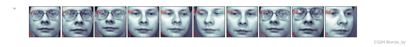
上图中的图像编号8带有眼镜，并且被分类为无眼镜。
如果我们看一下这个例子，我们可以看到它与其他带眼镜的图像不同（眼镜的边框看不清楚，人闭着眼睛），这可能就是它误判的原因。

我们创建了一个带有线性 SVM 模型的人脸分类器。
通常我们在第一次试验中不会得到如此好的结果。在这些情况下（除了查看不同的特征），我们可以开始调整算法的超参数。
在 SVM 的特定情况下，我们可以尝试不同的核函数；如果线性没有给出好的结果，我们可以尝试使用多项式或 RBF 核。此外，C和gamma参数可能会影响结果。
'''
[y_pred,y_test]

[array([1., 1., 1., 0., 0., 0., 0., 1., 0., 0.]),
 array([1., 1., 1., 0., 0., 0., 0., 1., 1., 0.])]