支持向量机svm分类、回归、网格搜索 基于sklearn(python)实现

前言

由于水平有限 支持向量机（support vector machine）的数学原理和证明就不讲了 想知道可以去看李航的机器学习或者西瓜书

---

svm的一般步骤

• 1、读入数据，将数据调成该库能够识别的格式
• 2、将数据标准化，防止样本中不同特征的数值差别较大，对分类结果产生较大影响
• 3、利用网格搜索和k折交叉验证选择最优参数C、γ与核函数的组合
• 4、使用最优参数来训练模型；
• 5、测试得到的分类器。

---

一、核函数介绍

一些线性不可分的问题可能是非线性可分的，即特征空间存在超曲面（hypersurface）将正类和负类分开。
也就是在二维下，我们无法用直线将两类分开
在三维下，我们无法用平面将两类分开
在更高维度下，我们无法用超平面将两类分开
而使用非线性函数可以将非线性可分问题从原始的特征空间映射至更高维的希尔伯特空间（Hilbert space） ，从而转化为线性可分问题
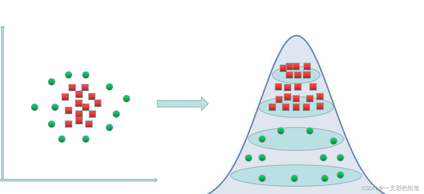
举一个二维可视化的例子，如下图
下图左边无法用直线将红绿两类完全分开，于是乎我们利用核函数将他们升维，像下图就是映射到一个高斯分布了，最后做到了超曲面分类的效果

---

二、交叉检验的介绍

具体分为简单交叉检验以及k折交叉验证

• 简单交叉检验
  方法:将原始数据随机划分成训练集和测试集两部分
  比如说，将样本按照70%和30%的比例分成两部分，70%的样本用于训练数据，30%样本用于模型验证。
  缺点:(1)数据都只被用了一次，没有被充分利用
  (2) 测试集上计算出来的最后评估指标与原始分组有很大关系
• k折交叉检验(k-ford交叉检验)
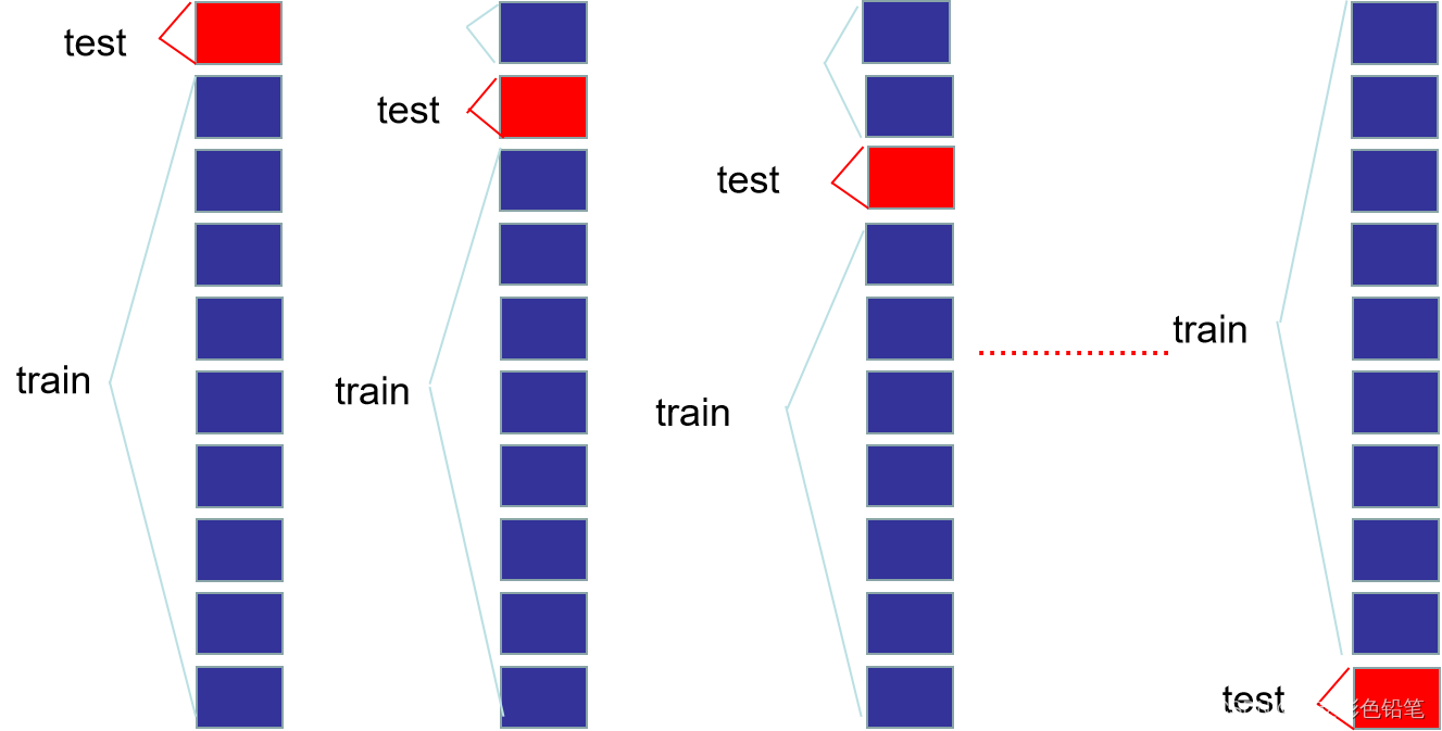
  举个例子，这里取k=10
  (1)将原始数据分成10份
  (2)依次将其中一份作为测试集，其余九份作为训练集，这样就依次计算十次
  (3)最后计算10次计算所得分类率的平均值，作为该模型的真实分类率
  如下图
  

---

三、具体代码实现

核心函数 class sklearn.svm.SVC 与 class sklearn.svm.SVR

class sklearn.svm.SVC(
C=1.0,             #错误样本的惩罚参数
kernel='rbf',      #适用何种核函数算法。 linear线性、poly多项式、rbf高斯、sigmoid、precomputed自定义,
degree=3,          #多项式核函数的阶数
gamma='auto',      #当kernel为'rbf','poly'或'sigmoid'时的kernel系数。默认是'auto',则会选择 1/n_features(特征数的倒数) 
coef0=0.0,         #kernel函数的常数项
shrinking=True,    #是否采用shrinking heuristic方法，默认为true
probability=False, #是否估计概率，会增加计算时间
tol=0.001,         #误差项达到指定值时则停止训练，默认为0.001
cache_size=200,    #核函数cache缓存大小，默认为200
class_weight=None, #类别的权重，字典形式传递。设置第几类的参数C为weight*C(C-SVC中的C)
verbose=False,     #允许冗余输出
max_iter=-1,       #最大迭代次数。-1为无限制。
decision_function_shape='ovr', #‘ovo’, ‘ovr’ or None, default=None3，ovo指一对一，ovr指一对剩余的(即其中一类作为第一类，其余作为第二类)
random_state=None  #数据乱序时的种子值，int类型
)
#因此，主要调节的参数有：C、kernel、degree、gamma、coef0。
#类的属性 support_vectors 支持向量、  support_ 支持向量的索引、  n_support_ 个数
#类的方法 基本差不多

---

svm分类

from sklearn.svm import SVC
from sklearn.preprocessing import StandardScaler #可做标准化
from sklearn.model_selection import train_test_split

#读入数据
import pandas as pd
import numpy as np
import matplotlib.pylab as plt
df=pd.read_excel(r'C:\Users\王金鹏\Desktop\决策树与随机森林.xlsx')
x=df.iloc[:,1:5]
y=df['目标']
#标准化
std=StandardScaler()
x_std=std.fit_transform(x)
#拆分训练集
x_train, x_test, y_train, y_test= train_test_split(x_std,y,train_size=0.75)
#svm建模
svm_classification =SVC()
svm_classification.fit(x_train,y_train)
#模型效果
print(svm_classification.score(x_test,y_test))

---

svm回归

from sklearn.svm import SVR
from sklearn.preprocessing import StandardScaler #可做标准化
from sklearn.model_selection import train_test_split

#读入数据
import pandas as pd
import numpy as np
import matplotlib.pylab as plt
df=pd.read_excel(r'C:\Users\王金鹏\Desktop\决策树与随机森林.xlsx')
x=df.iloc[:,1:5]
y=df['目标']
#标准化
std=StandardScaler()
x_std=std.fit_transform(x)
#拆分训练集
x_train, x_test, y_train, y_test= train_test_split(x_std,y,train_size=0.75)
#svm建模
svm_regression = SVR()
svm_regression.fit(x_train,y_train)
#模型效果
print(svm_regression.score(x_test,y_test))

---

网格搜索与k折交叉验证

• 网格搜索：在参数的排列组合中，找到最好的参数组合

from sklearn.model_selection import GridSearchCV
#定义参数的组合
params={
    
    
'kernel':('linear','rbf','poly'),
'C':[0.01,0.1,0.5,1,2,10,100]
}
# 用网格搜索方式拟合模型
model = GridSearchCV(svm_classification,param_grid=params,cv=10)
model.fit(x_std,y)
#查看结果
print("最好的参数组合: ",model.best_params_)
print("最好的score: ",model.best_score_)

• 运行结果
  

---

类别预测

先用网格搜索寻找最优参数，然后使用最优参数进行svm预测

from sklearn.model_selection import GridSearchCV
#定义参数的组合
params={
    
    
'kernel':('linear','rbf','poly'),
'C':[0.001,0.01,0.1,0.5,1,2,10,100,1000,10000]
}
# 用网格搜索方式拟合模型
svm_classification =SVC()
model = GridSearchCV(svm_classification,param_grid=params,cv=10)
#这边数据的单位都是%  属于同一数量级，就不需要进行标准化了
x=df.iloc[:,1:5]
y=df['目标']
model.fit(x,y)
#查看结果
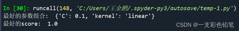
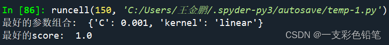
print("最好的参数组合: ",model.best_params_)
print("最好的score: ",model.best_score_)

网格搜索结果

进行预测

#这边数据的单位都是%  属于同一数量级，就不需要进行标准化了
x=df.iloc[:,1:5]
y=df['目标']
svm_clf = SVC(C=0.001,kernel='linear')
svm_clf.fit(x,y)
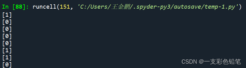
#A1 的预测
print(svm_clf.predict([[0,0,78.45,0]]))
#A2 的预测
print(svm_clf.predict([[34.3,0,37.75,0]]))
#A3 的预测
print(svm_clf.predict([[39.58,4.69,31.95,1.36]]))
#A4 的预测
print(svm_clf.predict([[24.28,8.31,35.47,0.79]]))
#A5 的预测
print(svm_clf.predict([[12.23,2.16,64.29,0.37]]))
#A6 的预测
print(svm_clf.predict([[0,0,93.17,1.35]]))
#A7 的预测
print(svm_clf.predict([[0,0,90.83,0.98]]))
#A8 的预测
print(svm_clf.predict([[21.24,11.34,51.12,0.23]]))

该题对应2022数模国赛C题的预测

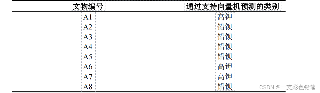
与官方所给的分类结果一致