SVM训练莺尾花数据集

SVM训练莺尾花数据集

代码在莺尾花数据集上训练SVM，数据集由莺尾花的测量值及其相应的物种标签组成。该模型使用70%数据用于训练，然后剩余部分进行测试。其中${}^{\prime }fi{t}^{\prime }$方法在训练集上训练数据，${}^{\prime }scor{e}^{\prime }$数据在返回模型的测试数据上的准确性：

注：其实这篇文章完全由openAI的chatGPT完成，包括代码部分，这里我将生成的英文原意和中文翻译都进行展示

代码

代码如下：

import numpy as np
from sklearn import datasets
from sklearn.svm import SVC
from sklearn.model_selection import train_test_split
import matplotlib.pyplot as plt

# Load the iris dataset
iris = datasets.load_iris()
X = iris["data"]
y = iris["target"]

# Split the data into training and test sets
X_train, X_test, y_train, y_test = train_test_split(X, y, test_size=0.3)

# Create the SVM model
model = SVC()

# Train the model on the training data
model.fit(X_train, y_train)

# Test the model on the test data
accuracy = model.score(X_test, y_test)

# Print the test accuracy
print("Test accuracy: {:.2f}".format(accuracy))

# Plot the data
fig, ax = plt.subplots()
colors = ["r", "g", "b"]
for i in range(3):
    indices = np.where(y == i)[0]
    ax.scatter(X[indices, 0], X[indices, 1], c=colors[i], label=iris["target_names"][i])
ax.legend()
plt.show()

---

代码相关解释

---

代码解释

import numpy as np
from sklearn import datasets
from sklearn.svm import SVC
from sklearn.model_selection import train_test_split
import matplotlib.pyplot as plt

在这些行中，我们导入必要的库。numpy是 Python 中用于科学计算的库，我们将使用它来存储和操作数据。datasets是scikit-learn库中的一个模块，其中包含许多可用于机器学习的数据集，我们将使用它来加载鸢尾花数据集。SVC是scikit-learn库中支持向量机 (SVM) 的类，我们将使用它来创建 SVM 模型。是我们将用于将数据拆分为训练集和测试集的模块中的train_test_split一个函数。最后，是库中的一个模块，我们将使用它来绘制数据。model_selection，scikit-learn，pyplot，matplotlib

# Load the iris dataset
iris = datasets.load_iris()
X = iris["data"]
y = iris["target"]

在这些行中，我们从模块加载 iris 数据集datasets并将其存储在一个名为iris. 鸢尾花数据集是一个类似字典的对象，其中包含数据和数据标签。我们将数据存储在一个名为 的变量X中，将标签存储在一个名为 的变量中y。数据由每个样本的四个特征（萼片长度、萼片宽度、花瓣长度和花瓣宽度）组成，标签是对应的鸢尾属植物属性

# Split the data into training and test sets
X_train, X_test, y_train, y_test = train_test_split(X, y, test_size=0.3)

在这一行中，我们使用该train_test_split函数将数据和标签拆分为训练集和测试集。该test_size参数指定应该用于测试的数据部分。在这种情况下，我们使用 30% 的数据进行测试，70% 的数据用于训练。该函数返回四个数组：X_trainandy_train包含训练数据和标签，X_test和y_test包含测试数据和标签。

# Create the SVM model
model = SVC()

SVC在这一行中，我们使用该类创建一个 SVM 模型。我们不需要指定任何参数，因此我们可以像调用函数一样简单地创建类的实例

# Train the model on the training data
model.fit(X_train, y_train)

在这一行中，我们使用对象的fit方法model在训练数据上训练模型。该方法有两个参数：数据和标签。

# Test the model on the test data
accuracy = model.score(X_test, y_test)

# Print the test accuracy
print("Test accuracy: {:.2f}".format(accuracy))

在这些行中，我们使用对象的score方法model来评估模型在测试数据上的准确性。该方法有两个参数：测试数据和测试标签。它返回一个介于 0 和 1 之间的浮点数，其中 1 表示完美的精度。我们使用字符串格式将准确性打印到控制台。

# Plot the data
fig, ax = plt.subplots()
colors = ["r", "g", "b"]
for i in range(3):
    indices = np.where(y == i)[0]
    ax.scatter(X[indices, 0], X[indices, 1], c=colors[i], label=iris["target_names"][i])
ax.legend()
plt.show()

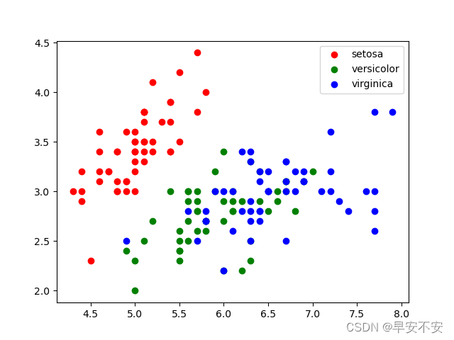
在这些行中，我们使用subplots函数 frommatplotlib创建一个图形和一个轴对象，然后我们使用scatter轴对象的方法绘制数据。我们遍历三种鸢尾，对于每个物种，我们使用where函数 from选择具有相应标签的样本numpy。然后我们使用该方法绘制这些样本scatter，其中萼片长度为 x 轴，萼片宽度为 y 轴。我们为每个物种使用不同的颜色，并使用该legend方法向图中添加图例。最后，我们使用show函数来显示绘图。

---

原文

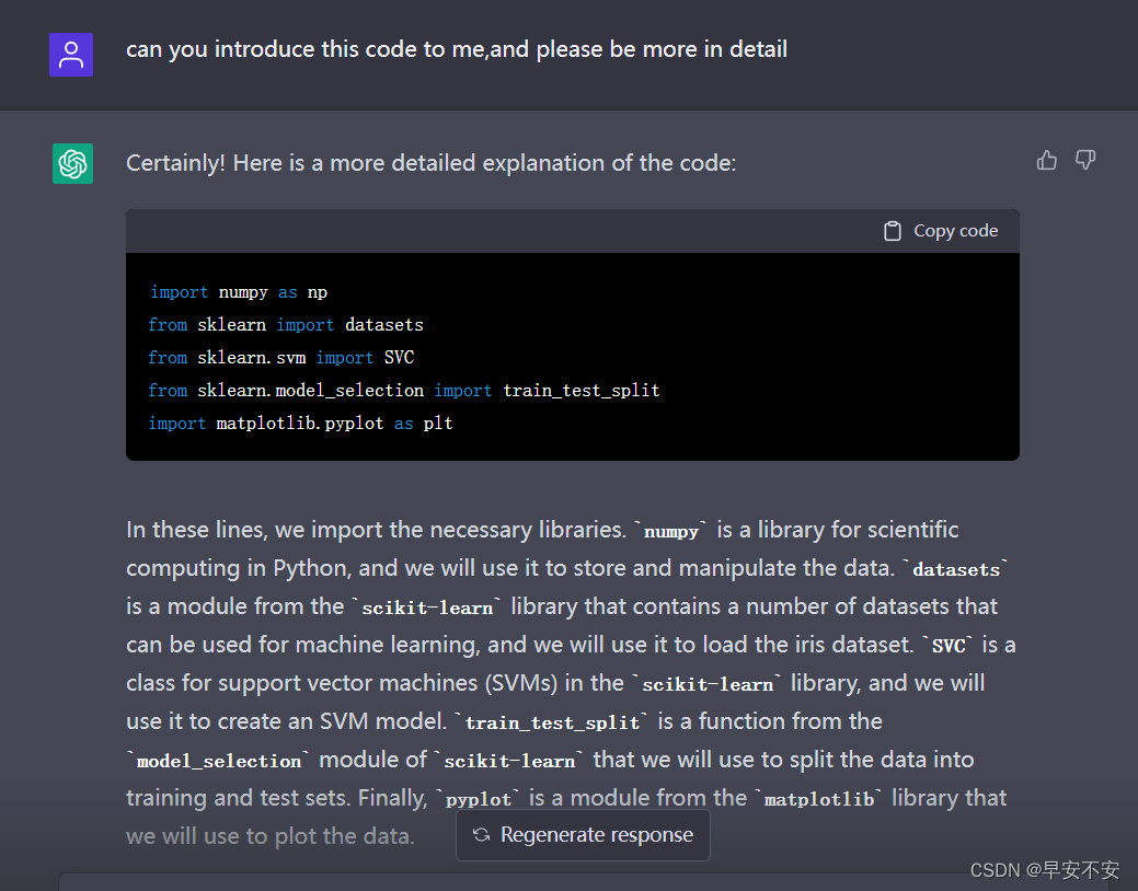
Certainly! Here is a more detailed explanation of the code:

import numpy as np
from sklearn import datasets
from sklearn.svm import SVC
from sklearn.model_selection import train_test_split
import matplotlib.pyplot as plt

In these lines, we import the necessary libraries. numpy is a library for scientific computing in Python, and we will use it to store and manipulate the data. datasets is a module from the scikit-learn library that contains a number of datasets that can be used for machine learning, and we will use it to load the iris dataset. SVC is a class for support vector machines (SVMs) in the scikit-learn library, and we will use it to create an SVM model. train_test_split is a function from the model_selection module of scikit-learn that we will use to split the data into training and test sets. Finally, pyplot is a module from the matplotlib library that we will use to plot the data.

# Load the iris dataset
iris = datasets.load_iris()
X = iris["data"]
y = iris["target"]

In these lines, we load the iris dataset from the datasets module and store it in a variable called iris. The iris dataset is a dictionary-like object that contains the data and the labels for the data. We store the data in a variable called X, and the labels in a variable called y. The data consists of four features for each sample (sepal length, sepal width, petal length, and petal width), and the labels are the corresponding species of iris

# Split the data into training and test sets
X_train, X_test, y_train, y_test = train_test_split(X, y, test_size=0.3)

In this line, we use the train_test_split function to split the data and labels into training and test sets. The test_size argument specifies the fraction of the data that should be used for testing. In this case, we are using 30% of the data for testing and 70% for training. The function returns four arrays: X_train and y_train contain the training data and labels, and X_test and y_test contain the test data and labels.

# Create the SVM model
model = SVC()

In this line, we create an SVM model using the SVC class. We don’t need to specify any arguments, so we can simply create an instance of the class by calling it like a function.

# Train the model on the training data
model.fit(X_train, y_train)

In this line, we use the fit method of the model object to train the model on the training data. The method takes two arguments: the data and the labels.

# Test the model on the test data
accuracy = model.score(X_test, y_test)

# Print the test accuracy
print("Test accuracy: {:.2f}".format(accuracy))

In these lines, we use the score method of the model object to evaluate the accuracy of the model on the test data. The method takes two arguments: the test data and the test labels. It returns a floating point number between 0 and 1, where 1 represents perfect accuracy. We print the accuracy to the console using string formatting.

# Plot the data
fig, ax = plt.subplots()
colors = ["r", "g", "b"]
for i in range(3):
    indices = np.where(y == i)[0]
    ax.scatter(X[indices, 0], X[indices, 1], c=colors[i], label=iris["target_names"][i])
ax.legend()
plt.show()

In these lines, we use the subplots function from matplotlib to create a figure and an axis object, and then we use the scatter method of the axis object to plot the data. We loop over the three species of iris, and for each species, we select the samples that have the corresponding label using the where function from numpy. We then plot these samples using the scatter method, with the sepal length as the x-axis and the sepal width as the y-axis. We use different colors for each species, and we add a legend to the plot using the legend method. Finally, we use the show function to display the plot.