前言
- 在时间序列模型中WaveNet模型在某些数据集上的表现比LSTM要更好,经常打Kaggle比赛的算法训练师应该有所了解。
- 关于WaveNet模型的理论在这里就不讲了,如果大家感兴趣可以读一下WaveNet论文
- GluonTs包中内置了WaveNet模型,本篇论文将示例如何使用WaveNet模型训练自己的数据,并作出预测,代码我都做了注释。
- 首先确保GluonTs包已经安装,这里建议安装
torch版本,!pip install "gluonts[torch,pro]" - 参考资料:GluonTs官网
训练WaveNet模型
导入包
#加载包
import numpy as np
import pandas as pd
from plotnine import*
import seaborn as sns
from scipy import stats

import matplotlib as mpl
import matplotlib.pyplot as plt
#中文显示问题
plt.rcParams['font.sans-serif']=['SimHei']
plt.rcParams['axes.unicode_minus'] = False

# notebook嵌入图片
%matplotlib inline
# 提高分辨率
%config InlineBackend.figure_format='retina'

# 切分数据
from sklearn.model_selection import train_test_split
# 评价指标
from sklearn.metrics import mean_squared_error

# 忽略警告
import warnings
warnings.filterwarnings('ignore')

# GluonTs包
from gluonts.dataset.util import to_pandas
from gluonts.dataset.common import ListDataset
from gluonts.dataset.split import split
from gluonts.model.wavenet import WaveNetEstimator
from gluonts.evaluation import Evaluator
from gluonts.mx import Trainer
import optuna
import json
导入数据
df = pd.read_csv('Prophet.csv',encoding='utf-8')
# 将日期列转化为时间格式
df.loc[:,'时间'] = pd.to_datetime(df.loc[:,'时间'].astype(str), format='%Y/%m/%d %H:%M:%S', errors='coerce')
# 一定要检查时间完整性,否则会报freq错误
df.head()
- 将数据转换为GluonTs包内置数据类型
ListDataset - 我需要预测后面960个时间长度,并且数据时间间隔为15分钟
# 预测长度
prediction_length = 960
# 时间间隔
freq = '15T'
train_ds = ListDataset([{

    "start":df.iloc[0,0],
                         "target":df['总有功功率(kw)']}],freq=freq)
模型建立与训练
- 模型有很多参数可以调整,具体可以参考官方API,这里只是做简单演示。
wave = WaveNetEstimator(freq = freq,prediction_length = prediction_length,trainer=Trainer(epochs=5))
model = wave.train(train_ds)
预测
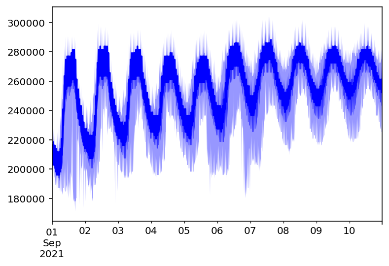
- 使用模型预测,并绘制图像保存。
prediction = next(model.predict(train_ds))
# print(prediction.mean)
prediction.plot(output_file='graph.png')
模型调优
- 在GluonTs包中集成了
optuna工具,用于参数调优。optuna的使用方法,可以查阅opturna帮助文档 - 首先将数据格式由DataEntry转换为DataFrame格式
# 将DataEntry转换为DataFrame格式
def dataentry_to_dataframe(entry):
    df = pd.DataFrame(
        entry["target"],
        columns=[entry.get("item_id")],
        index=pd.period_range(
            start=entry["start"], periods=len(entry["target"]), freq=entry["start"].freq
        ),
    )

    return df
- 定义模型优化类,有不懂可以看注释,写的应该很详细
class WaveNetTuning:
    def __init__(
        # 传入数据、预测长度、时间间隔、模型效果衡量指标
        self, dataset, prediction_length, freq, metric_type="mean_wQuantileLoss"
    ):
        self.dataset = dataset
        self.prediction_length = prediction_length
        self.freq = freq
        self.metric_type = metric_type

        # 分隔训练集、验证集、测试集
        self.train, test_template = split(dataset, offset=-self.prediction_length)
        validation = test_template.generate_instances(
            prediction_length=prediction_length
        )
        self.validation_input = [entry[0] for entry in validation]
        self.validation_label = [
            dataentry_to_dataframe(entry[1]) for entry in validation
        ]

    def get_params(self, trial) -> dict:
        # 需要调整的参数,suggest_float指明参数为浮点数,suggest_int指明参数为整型
        return {


            "learning_rate": trial.suggest_float("learning_rate", 1e-3, 1e-2),
            "epochs": trial.suggest_int("epochs", 5, 20),
        }

    def __call__(self, trial):
        # 将参数传入字典
        params = self.get_params(trial)
        # 定义模型
        estimator = WaveNetEstimator(
            prediction_length=self.prediction_length,
            freq=self.freq,
            trainer=Trainer(epochs=params["epochs"],learning_rate = params["learning_rate"])
        )

        # 训练函数
        predictor = estimator.train(self.train, cache_data=True)
        # 在验证集上检验模型效果
        forecast_it = predictor.predict(self.validation_input)

        forecasts = list(forecast_it)

        # 设定需要计算的分位数
        evaluator = Evaluator(quantiles=[0.1, 0.5, 0.9])
        agg_metrics, item_metrics = evaluator(
            self.validation_label, forecasts, num_series=len(self.dataset)
        )
        # 返回模型误差
        return agg_metrics[self.metric_type]
- 设定优化类型,建立优化器,开始优化
import time
# 记录开始时间
start_time = time.time()
# 优化类型为最小化
study = optuna.create_study(direction="minimize")
# 开始优化,n_trials为迭代次数,次数越多找到最优参数的概率越大
study.optimize(WaveNetTuning(train_ds, prediction_length = prediction_length, freq = freq),
    n_trials=5)

# 信息输出
print("Number of finished trials: {}".format(len(study.trials)))

print("Best trial:")
trial = study.best_trial

print("  Value: {}".format(trial.value))

print("  Params: ")
for key, value in trial.params.items():
    print("    {}: {}".format(key, value))
print(time.time() - start_time)
输出:
[I 2022-10-25 10:10:35,163] A new study created in memory with name: no-name-52f5c55b-2016-4332-b284-bed5ed00ecae
  0%|          | 0/50 [00:00<?, ?it/s][10:10:46] ../src/operator/nn/./cudnn/./cudnn_algoreg-inl.h:96: Running performance tests to find the best convolution algorithm, this can take a while... (set the environment variable MXNET_CUDNN_AUTOTUNE_DEFAULT to 0 to disable)
100%|██████████| 50/50 [00:25<00:00,  1.94it/s, epoch=1/9, avg_epoch_loss=4.45]
100%|██████████| 50/50 [00:14<00:00,  3.47it/s, epoch=2/9, avg_epoch_loss=3.03]
100%|██████████| 50/50 [00:14<00:00,  3.43it/s, epoch=3/9, avg_epoch_loss=2.34]
100%|██████████| 50/50 [00:14<00:00,  3.45it/s, epoch=4/9, avg_epoch_loss=2.1]
100%|██████████| 50/50 [00:14<00:00,  3.43it/s, epoch=5/9, avg_epoch_loss=1.93]
100%|██████████| 50/50 [00:14<00:00,  3.46it/s, epoch=6/9, avg_epoch_loss=1.84]
100%|██████████| 50/50 [00:14<00:00,  3.41it/s, epoch=7/9, avg_epoch_loss=1.81]
100%|██████████| 50/50 [00:14<00:00,  3.46it/s, epoch=8/9, avg_epoch_loss=1.73]
100%|██████████| 50/50 [00:14<00:00,  3.47it/s, epoch=9/9, avg_epoch_loss=1.69]
[10:13:04] ../src/operator/nn/./cudnn/./cudnn_algoreg-inl.h:96: Running performance tests to find the best convolution algorithm, this can take a while... (set the environment variable MXNET_CUDNN_AUTOTUNE_DEFAULT to 0 to disable)
Running evaluation: 100%|██████████| 1/1 [00:00<00:00, 14.15it/s]
[I 2022-10-25 10:13:22,629] Trial 0 finished with value: 0.05870472306833338 and parameters: {

    'learning_rate': 0.0065477390193292885, 'epochs': 9}. Best is trial 0 with value: 0.05870472306833338.
100%|██████████| 50/50 [00:14<00:00,  3.38it/s, epoch=1/6, avg_epoch_loss=4.36]
100%|██████████| 50/50 [00:14<00:00,  3.46it/s, epoch=2/6, avg_epoch_loss=3.13]
100%|██████████| 50/50 [00:14<00:00,  3.47it/s, epoch=3/6, avg_epoch_loss=2.31]
100%|██████████| 50/50 [00:14<00:00,  3.46it/s, epoch=4/6, avg_epoch_loss=2.06]
100%|██████████| 50/50 [00:14<00:00,  3.44it/s, epoch=5/6, avg_epoch_loss=1.89]
100%|██████████| 50/50 [00:14<00:00,  3.44it/s, epoch=6/6, avg_epoch_loss=1.8]
Running evaluation: 100%|██████████| 1/1 [00:00<00:00, 15.79it/s]
[I 2022-10-25 10:15:07,403] Trial 1 finished with value: 0.03777278966320785 and parameters: {

    'learning_rate': 0.00816750948981148, 'epochs': 6}. Best is trial 1 with value: 0.03777278966320785.
100%|██████████| 50/50 [00:14<00:00,  3.36it/s, epoch=1/9, avg_epoch_loss=4.65]
100%|██████████| 50/50 [00:14<00:00,  3.48it/s, epoch=2/9, avg_epoch_loss=3.58]
100%|██████████| 50/50 [00:14<00:00,  3.43it/s, epoch=3/9, avg_epoch_loss=2.61]
100%|██████████| 50/50 [00:14<00:00,  3.46it/s, epoch=4/9, avg_epoch_loss=2.21]
100%|██████████| 50/50 [00:14<00:00,  3.41it/s, epoch=5/9, avg_epoch_loss=2.05]
100%|██████████| 50/50 [00:14<00:00,  3.46it/s, epoch=6/9, avg_epoch_loss=1.94]
100%|██████████| 50/50 [00:14<00:00,  3.43it/s, epoch=7/9, avg_epoch_loss=1.86]
100%|██████████| 50/50 [00:14<00:00,  3.50it/s, epoch=8/9, avg_epoch_loss=1.86]
100%|██████████| 50/50 [00:14<00:00,  3.42it/s, epoch=9/9, avg_epoch_loss=1.77]
Running evaluation: 100%|██████████| 1/1 [00:00<00:00, 14.50it/s]
[I 2022-10-25 10:17:35,808] Trial 2 finished with value: 0.03438310304130423 and parameters: {

    'learning_rate': 0.004057893781175508, 'epochs': 9}. Best is trial 2 with value: 0.03438310304130423.
100%|██████████| 50/50 [00:14<00:00,  3.37it/s, epoch=1/13, avg_epoch_loss=5.18]
100%|██████████| 50/50 [00:14<00:00,  3.45it/s, epoch=2/13, avg_epoch_loss=4.23]
100%|██████████| 50/50 [00:14<00:00,  3.47it/s, epoch=3/13, avg_epoch_loss=3.82]
100%|██████████| 50/50 [00:14<00:00,  3.45it/s, epoch=4/13, avg_epoch_loss=3.22]
100%|██████████| 50/50 [00:14<00:00,  3.45it/s, epoch=5/13, avg_epoch_loss=2.64]
100%|██████████| 50/50 [00:14<00:00,  3.45it/s, epoch=6/13, avg_epoch_loss=2.36]
100%|██████████| 50/50 [00:14<00:00,  3.50it/s, epoch=7/13, avg_epoch_loss=2.22]
100%|██████████| 50/50 [00:14<00:00,  3.46it/s, epoch=8/13, avg_epoch_loss=2.11]
100%|██████████| 50/50 [00:14<00:00,  3.48it/s, epoch=9/13, avg_epoch_loss=2.06]
100%|██████████| 50/50 [00:14<00:00,  3.43it/s, epoch=10/13, avg_epoch_loss=1.97]
100%|██████████| 50/50 [00:14<00:00,  3.46it/s, epoch=11/13, avg_epoch_loss=2]
100%|██████████| 50/50 [00:14<00:00,  3.43it/s, epoch=12/13, avg_epoch_loss=1.92]
100%|██████████| 50/50 [00:14<00:00,  3.48it/s, epoch=13/13, avg_epoch_loss=1.87]
Running evaluation: 100%|██████████| 1/1 [00:00<00:00, 13.78it/s]
[I 2022-10-25 10:21:02,493] Trial 3 finished with value: 0.04105908616187858 and parameters: {

    'learning_rate': 0.00130586676867756, 'epochs': 13}. Best is trial 2 with value: 0.03438310304130423.
100%|██████████| 50/50 [00:14<00:00,  3.42it/s, epoch=1/20, avg_epoch_loss=5.42]
100%|██████████| 50/50 [00:14<00:00,  3.43it/s, epoch=2/20, avg_epoch_loss=4.22]
100%|██████████| 50/50 [00:14<00:00,  3.48it/s, epoch=3/20, avg_epoch_loss=3.89]
100%|██████████| 50/50 [00:14<00:00,  3.45it/s, epoch=4/20, avg_epoch_loss=3.52]
100%|██████████| 50/50 [00:14<00:00,  3.47it/s, epoch=5/20, avg_epoch_loss=3.07]
100%|██████████| 50/50 [00:14<00:00,  3.48it/s, epoch=6/20, avg_epoch_loss=2.64]
100%|██████████| 50/50 [00:14<00:00,  3.44it/s, epoch=7/20, avg_epoch_loss=2.4]
100%|██████████| 50/50 [00:14<00:00,  3.46it/s, epoch=8/20, avg_epoch_loss=2.25]
100%|██████████| 50/50 [00:14<00:00,  3.41it/s, epoch=9/20, avg_epoch_loss=2.16]
100%|██████████| 50/50 [00:14<00:00,  3.47it/s, epoch=10/20, avg_epoch_loss=2.11]
100%|██████████| 50/50 [00:14<00:00,  3.46it/s, epoch=11/20, avg_epoch_loss=2.04]
100%|██████████| 50/50 [00:14<00:00,  3.44it/s, epoch=12/20, avg_epoch_loss=1.99]
100%|██████████| 50/50 [00:14<00:00,  3.45it/s, epoch=13/20, avg_epoch_loss=1.98]
100%|██████████| 50/50 [00:14<00:00,  3.47it/s, epoch=14/20, avg_epoch_loss=1.92]
100%|██████████| 50/50 [00:14<00:00,  3.44it/s, epoch=15/20, avg_epoch_loss=1.88]
100%|██████████| 50/50 [00:14<00:00,  3.49it/s, epoch=16/20, avg_epoch_loss=1.85]
100%|██████████| 50/50 [00:14<00:00,  3.48it/s, epoch=17/20, avg_epoch_loss=1.82]
100%|██████████| 50/50 [00:14<00:00,  3.44it/s, epoch=18/20, avg_epoch_loss=1.79]
100%|██████████| 50/50 [00:14<00:00,  3.50it/s, epoch=19/20, avg_epoch_loss=1.8]
100%|██████████| 50/50 [00:14<00:00,  3.48it/s, epoch=20/20, avg_epoch_loss=1.76]
Running evaluation: 100%|██████████| 1/1 [00:00<00:00, 15.14it/s]
[I 2022-10-25 10:26:09,543] Trial 4 finished with value: 0.0251484216989744 and parameters: {

    'learning_rate': 0.0010629028925384662, 'epochs': 20}. Best is trial 4 with value: 0.0251484216989744.
Number of finished trials: 5
Best trial:
  Value: 0.0251484216989744
  Params:
    learning_rate: 0.0010629028925384662
    epochs: 20
934.3837442398071
- 获得最优参后再次训练模型
wave = WaveNetEstimator(freq = freq,prediction_length = prediction_length,trainer=Trainer(epochs=trial.params["epochs"],learning_rate = trial.params["learning_rate"]))
model = wave.train(train_ds)
输出:
100%|██████████| 50/50 [02:49<00:00,  3.38s/it, epoch=1/20, avg_epoch_loss=5.3]
100%|██████████| 50/50 [02:37<00:00,  3.15s/it, epoch=2/20, avg_epoch_loss=4.19]
100%|██████████| 50/50 [02:48<00:00,  3.38s/it, epoch=3/20, avg_epoch_loss=3.81]
100%|██████████| 50/50 [02:43<00:00,  3.26s/it, epoch=4/20, avg_epoch_loss=3.3]
100%|██████████| 50/50 [02:32<00:00,  3.05s/it, epoch=5/20, avg_epoch_loss=2.76]
100%|██████████| 50/50 [02:43<00:00,  3.28s/it, epoch=6/20, avg_epoch_loss=2.47]
100%|██████████| 50/50 [02:42<00:00,  3.25s/it, epoch=7/20, avg_epoch_loss=2.29]
100%|██████████| 50/50 [02:39<00:00,  3.20s/it, epoch=8/20, avg_epoch_loss=2.18]
100%|██████████| 50/50 [02:43<00:00,  3.26s/it, epoch=9/20, avg_epoch_loss=2.12]
100%|██████████| 50/50 [02:43<00:00,  3.27s/it, epoch=10/20, avg_epoch_loss=2.07]
100%|██████████| 50/50 [02:40<00:00,  3.21s/it, epoch=11/20, avg_epoch_loss=2.01]
100%|██████████| 50/50 [02:37<00:00,  3.15s/it, epoch=13/20, avg_epoch_loss=1.93]
100%|██████████| 50/50 [02:34<00:00,  3.10s/it, epoch=14/20, avg_epoch_loss=1.91]
100%|██████████| 50/50 [02:42<00:00,  3.24s/it, epoch=15/20, avg_epoch_loss=1.85]
100%|██████████| 50/50 [02:39<00:00,  3.18s/it, epoch=16/20, avg_epoch_loss=1.85]
100%|██████████| 50/50 [02:39<00:00,  3.19s/it, epoch=18/20, avg_epoch_loss=1.8]
100%|██████████| 40/50 [02:15<00:33,  3.38s/it, epoch=20/20, avg_epoch_loss=1.77]
- 观察模型效果,注意这里的
train_ds函数会自动删除数据的最后960个点,比如train_ds有10000个样本,该函数会将前10000-960个数据作为输入,输出后960个点,以观察模型效果
from gluonts.evaluation import make_evaluation_predictions
forecast_it, ts_it = make_evaluation_predictions(
    dataset=train_ds, # 预测数据集(在训练数据中删除960个点)
    predictor=model,  # 最优模型
    num_samples=100,  # 采样点,用于快速固定模型架构
)
- 取得预测值以及对应分位数
forecasts = list(forecast_it)
tss = list(ts_it)
forecast_entry = forecasts[0]
ts_entry = tss[0]
- 绘图观察
def plot_prob_forecasts(ts_entry, forecast_entry):
    plot_length = 960
    prediction_intervals = (50.0, 90.0)
    legend = ["observations", "median prediction"] + [
        f"{

      k}% prediction interval" for k in prediction_intervals
    ][::-1]

    fig, ax = plt.subplots(1, 1, figsize=(10, 7))
    ts_entry[-plot_length:].plot(ax=ax)  # plot the time series
    forecast_entry.plot(prediction_intervals=prediction_intervals, color="g")
    plt.grid(which="both")
    plt.legend(legend, loc="upper left")
    plt.show()
- 可以看到模型预测值基本与实际值一致,或者说在分位数中基本包含。说明模型效果不错
# observations为真实值,median prediction为预测值,90%,50%预测值分位数
plot_prob_forecasts(ts_entry, forecast_entry)

- 输出模型评估指标
evaluator = Evaluator(quantiles=[0.1, 0.5, 0.9])
agg_metrics, item_metrics = evaluator(tss, forecasts)
print(json.dumps(agg_metrics, indent=4))
输出:
 "MSE": 559735876.2666667,
    "abs_error": 19179792.0,
    "abs_target_sum": 221908064.0,
    "abs_target_mean": 231154.23333333334,
    "seasonal_error": 7323.029618473895,
    "MASE": 2.7282355856650997,
    "MAPE": 0.09181206226348877,
    "sMAPE": 0.08502658208211263,
    "MSIS": 13.758000023993187,
    "QuantileLoss[0.1]": 10812644.68125,
    "Coverage[0.1]": 0.49895833333333334,
    "QuantileLoss[0.5]": 19179791.234375,
    "Coverage[0.5]": 0.9552083333333333,
    "QuantileLoss[0.9]": 6544961.284374999,
    "Coverage[0.9]": 0.9989583333333333,
    "RMSE": 23658.737841792547,
    "NRMSE": 0.10235044152393148,
    "ND": 0.08643125289939892,
    "wQuantileLoss[0.1]": 0.04872578529300314,
    "wQuantileLoss[0.5]": 0.08643124944920884,
    "wQuantileLoss[0.9]": 0.029494021832280053,
    "mean_absolute_QuantileLoss": 12179132.399999999,
    "mean_wQuantileLoss": 0.054883685524830673,
    "MAE_Coverage": 0.3177083333333333,
    "OWA": NaN
- 将所有数据作为输入,输出需要预测的后960个点
prediction = next(model.predict(train_ds))
# print(prediction.mean)
prediction.plot(output_file='graph.png')
结语
- 在模型调优这一块我仅仅优化了学习率和迭代次数,关于网络架构的参数优化因为时间问题,就没有过多说明,这里还是建议大家去读一下有关于WaveNet的论文,然后根据官方API对参数做进一步优化
- 训练时尽可能使用GPU,否则训练会很慢,时间成本会特别高