note
- 有了之前的数据分析,我们也根据数据集判断是监督学习还是无监督学习,并且根据我们的任务、数据样本量、特征稀疏性等进行判断使用什么模型。
- 模型指标:
- 准确率(precision)度量的是被预测为正例的样本中有多少是真正的正例
- 召回率(recall)度量的是正类样本中有多少被预测为正类
- f-分数是准确率与召回率的调和平均
文章目录
一、建立模型
下载sklearn的命令pip install scikit-learn。
from sklearn.model_selection import train_test_split
import pandas as pd
import numpy as np
import matplotlib.pyplot as plt
import seaborn as sns
from IPython.display import Image

plt.rcParams['font.sans-serif'] = ['SimHei']  # 用来正常显示中文标签
plt.rcParams['axes.unicode_minus'] = False  # 用来正常显示负号
plt.rcParams['figure.figsize'] = (10, 6)  # 设置输出图片大小
# 一般先取出X和y后再切割,有些情况会使用到未切割的,这时候X和y就可以用,x是清洗好的数据,y是我们要预测的存活数据'Survived'

data = pd.read_csv('clear_data.csv')
train = pd.read_csv('train.csv')
X = data
y = train['Survived']
# 对数据集进行切割, 留出法
X_train, X_test, y_train, y_test = train_test_split(X, y, stratify=y, random_state=0)
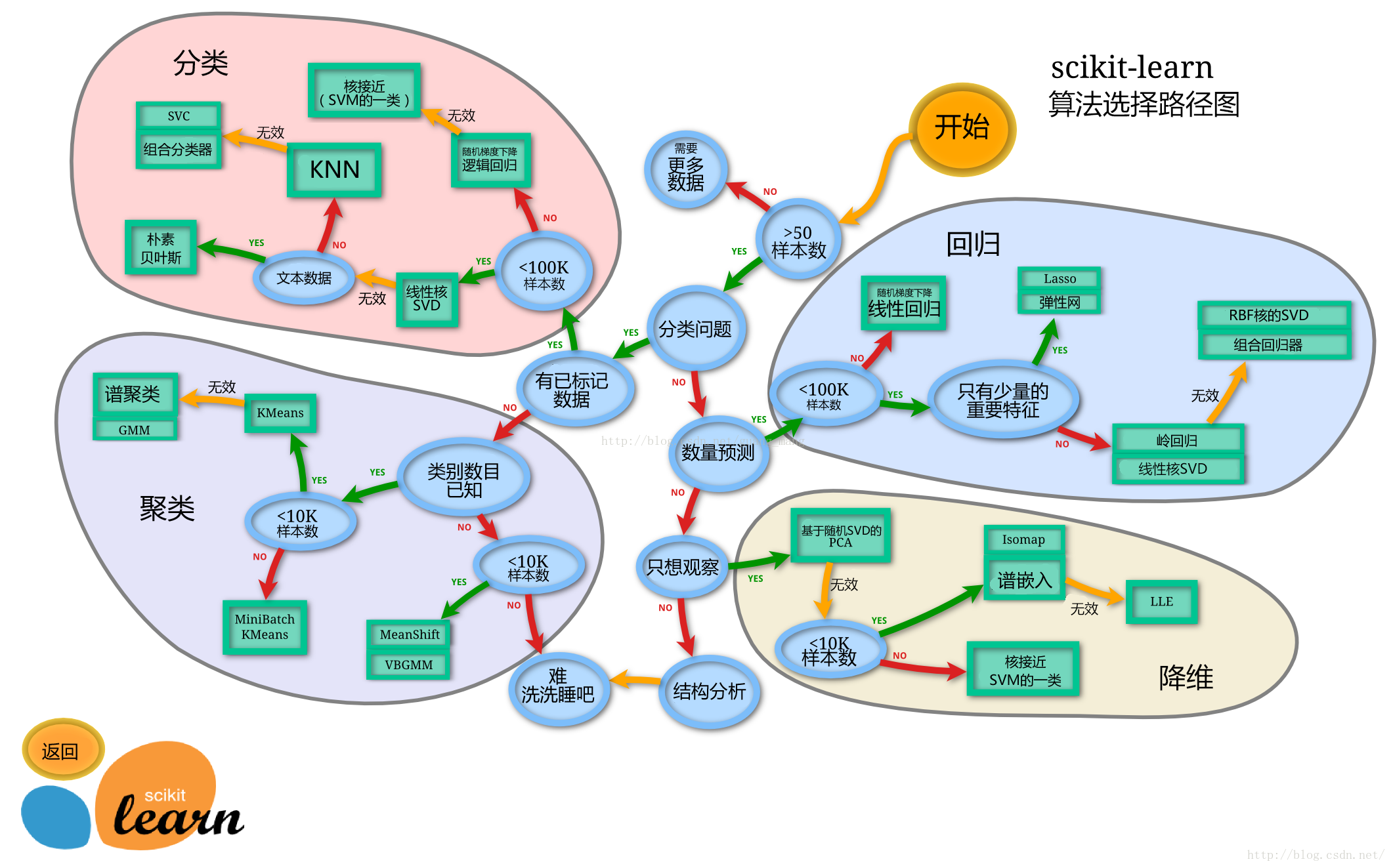
有了之前的数据分析,我们也根据数据集判断是监督学习还是无监督学习,并且根据我们的任务、数据样本量、特征稀疏性等进行判断使用什么模型。逻辑回归是分类模型,随机森林是决策树为了防止过拟合。通常会先用一个baseline作为基本模型,然后再选择其他泛化能力更强的模型(参考上图的算法选择路径,深度学习NN类模型的选择就更多了)。
from sklearn.linear_model import LogisticRegression
from sklearn.ensemble import RandomForestClassifier

# 1. 默认参数逻辑回归模型
lr = LogisticRegression()
lr.fit(X_train, y_train)
print("Training set score: {:.2f}".format(lr.score(X_train, y_train)))
print("Testing set score: {:.2f}".format(lr.score(X_test, y_test)))

# 2. 调整参数后的逻辑回归模型
lr2 = LogisticRegression(C=100)
lr2.fit(X_train, y_train)
print("Training set score: {:.2f}".format(lr2.score(X_train, y_train)))
print("Testing set score: {:.2f}".format(lr2.score(X_test, y_test)))

# 3. 默认参数的随机森林分类模型
rfc = RandomForestClassifier()
rfc.fit(X_train, y_train)
print("Training set score: {:.2f}".format(rfc.score(X_train, y_train)))
print("Testing set score: {:.2f}".format(rfc.score(X_test, y_test)))

# 4. 调整参数后的随机森林分类模型
rfc2 = RandomForestClassifier(n_estimators=100, max_depth=5)
rfc2.fit(X_train, y_train)
print("Training set score: {:.2f}".format(rfc2.score(X_train, y_train)))
print("Testing set score: {:.2f}".format(rfc2.score(X_test, y_test)))

# 5. 模型预测
pred = lr.predict(X_train)  # 预测标签
pred[:10]  # 显示前10个样本的预测结果
pred_proba = lr.predict_proba(X_train) # 预测标签概率

二、模型评估
- 模型评估是为了知道模型的泛化能力。
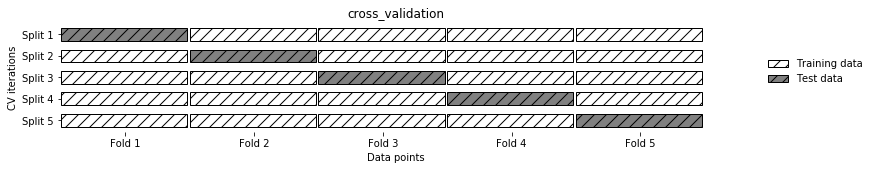
- 交叉验证(cross-validation)是一种评估泛化性能的统计学方法,它比单次划分训练集和测试集的方法更加稳定、全面。
- 在交叉验证中,数据被多次划分,并且需要训练多个模型。
- 最常用的交叉验证是 k 折交叉验证(k-fold cross-validation),其中 k 是由用户指定的数字,通常取 5 或 10。
模型指标:
- 准确率(precision)度量的是被预测为正例的样本中有多少是真正的正例
- 召回率(recall)度量的是正类样本中有多少被预测为正类
- f-分数是准确率与召回率的调和平均

2.1 交叉验证
十折交叉验证:
from sklearn.model_selection import cross_val_score
lr = LogisticRegression(C=100)
scores = cross_val_score(lr, X_train, y_train, cv=10)
# k折交叉验证分数, 这里是十折交叉验证
scores  # (10, )
# 平均交叉验证分数
print("Average cross-validation score: {:.2f}".format(scores.mean()))  # 0.79
2.2 混淆矩阵/recall/accuracy/F1
- 混淆矩阵的方法在sklearn中的
sklearn.metrics模块 - 混淆矩阵需要输入真实标签和预测标签
- 精确率、召回率以及f-分数可使用
classification_report模块
from sklearn.metrics import confusion_matrix
from sklearn.metrics import classification_report
# 训练模型
lr = LogisticRegression(C=100)
lr.fit(X_train, y_train)
pred = lr.predict(X_train)
# 混淆矩阵
confusion_matrix(y_train, pred)

# 精确率、召回率以及f1-score
print(classification_report(y_train, pred))

上面的左侧列0和1就是两个预测的标签,对应的不同预测指标。查准率和查全率是一对矛盾的指标,查全率recall衡量的是某标签的预测结果是否涵盖“周全”。
2.3 ROC曲线
ROC 曲线的横坐标是 False Positive Rate(FPR,假阳性率),纵坐标是 True Positive Rate (TPR,真阳性率)。 F P R a t e = F P N , T P R a t e = T P P \mathrm{FPRate}=\frac{\mathrm{FP}}{N}, T P Rate=\frac{\mathrm{TP}}{P} FPRate=NFP,TPRate=PTP
这里的P 指的是真实的正样本数量,N 是真实的负样本数量;TP 指的是 P 个正样本中被分类器预测为正样本的个数,FP 指的是 N 个负样本中被分类器预测为正样本的个数。

和 P-R 曲线一样,ROC 曲线也是通过不断移动模型正样本阈值生成的。如上面的动图,垂线其实就是我们的阈值,当垂线从右到左移动时,右边ROC曲线上的点,从下往上移动。如果来固定阈值,我们也可以看到左图中,其实和混淆矩阵中四个值是对应的:

from sklearn.metrics import roc_curve
fig = plt.figure(figsize=(4, 4))
fpr, tpr, thresholds = roc_curve(y_test, lr.decision_function(X_test))
plt.plot(fpr, tpr, label="ROC Curve")
plt.xlabel("FPR")
plt.ylabel("TPR (recall)")

# 找到最接近于0的阈值
close_zero = np.argmin(np.abs(thresholds))

plt.plot(fpr[close_zero],
		 tpr[close_zero],
		 'o',
		 markersize=10,
		 label="threshold zero",
		 fillstyle="none",
		 c='k',
		 mew=2)
plt.legend(loc=4)

三、Pyspark进行基础模型预测
在pyspark中使用mllib其实也是类似的,就是需要先将label和feature进行通过像StringIndexer和VectorIndexer转为模型输入前需要的格式,然后通过模型的定义后进行fit和transform操作。
# test libsvm dataset
#!usr/bin/env python
#encoding:utf-8
from __future__ import division
import findspark
findspark.init()
import pyspark
from pyspark import SparkConf
from pyspark.ml import Pipeline
from pyspark.context import SparkContext
from pyspark.sql.session import SparkSession
from pyspark.ml.classification import DecisionTreeClassifier
from pyspark.ml.evaluation import MulticlassClassificationEvaluator
from pyspark.ml.feature import StringIndexer, VectorIndexer,IndexToString

"""
conf=SparkConf().setAppName('MLDemo')
sc = SparkContext('local')
spark = SparkSession(sc)
"""

def gradientBoostedTreeClassifier(data="data/sample_libsvm_data.txt"):
    '''
    GBDT分类器
    '''
    #加载LIBSVM格式的数据集
    data = spark.read.format("libsvm").load(data)
    print("data数据集前5行:\n", data.show(n = 3))

    labelIndexer = StringIndexer(inputCol="label", outputCol="indexedLabel").fit(data)

    #自动识别类别特征并构建索引,指定maxCategories,因此具有> 4个不同值的特征被视为连续的
    featureIndexer=VectorIndexer(inputCol="features", outputCol="indexedFeatures", maxCategories=4).fit(data)

    #训练集、测试集划分
    (trainingData, testData) = data.randomSplit([0.7, 0.3])

    # 构建10个基分类器 maxIter = 10
    gbt = GBTClassifier(labelCol="indexedLabel", featuresCol="indexedFeatures", maxIter=10)

    pipeline = Pipeline(stages=[labelIndexer, featureIndexer, gbt])
    model = pipeline.fit(trainingData)
    # transformer是一个pipelineStage,将一个df转为另一个df,对testData进行
    predictions = model.transform(testData)

    #展示前5行数据,或者show进行打印
    predictions.select("prediction", "indexedLabel", "features").show(5)

    #展示预测标签与真实标签,计算测试误差
    evaluator = MulticlassClassificationEvaluator(
        labelCol="indexedLabel", predictionCol="prediction", metricName="accuracy")

    # 评估model
    accuracy = evaluator.evaluate(predictions)
    print("Test Error = %g" % (1.0 - accuracy))
    gbtModel = model.stages[2]
    print('gbtModelSummary: ',gbtModel)  #模型摘要


if __name__=='__main__':
    filepath = "file:///home/hadoop/development/RecSys/"
    gradientBoostedTreeClassifier(filepath + "data/sample_libsvm_data.txt")
pyspark适合数据量更大时候的模型预测,如GBDT结果如下:
+-----+--------------------+
|label|            features|
+-----+--------------------+
|  0.0|(692,[127,128,129...|
|  1.0|(692,[158,159,160...|
|  1.0|(692,[124,125,126...|
+-----+--------------------+
only showing top 3 rows

data数据集前5行:
 None
+----------+------------+--------------------+
|prediction|indexedLabel|            features|
+----------+------------+--------------------+
|       1.0|         1.0|(692,[95,96,97,12...|
|       1.0|         1.0|(692,[122,123,124...|
|       1.0|         1.0|(692,[124,125,126...|
|       1.0|         1.0|(692,[124,125,126...|
|       1.0|         1.0|(692,[125,126,127...|
+----------+------------+--------------------+
only showing top 5 rows

Test Error = 0.03125
gbtModelSummary:  GBTClassificationModel: uid = GBTClassifier_d0de0e9263e7, numTrees=10, numClasses=2, numFeatures=692
时间安排
| 任务 | 任务内容 | 时间 | 完成情况 |
|---|---|---|---|
| - | 1月16日周一开始 | ||
| Task01: | 数据加载及探索性数据分析(第一章第1,2,3节)(2天) | 16-17日周二 | 完成 |
| Task02: | 数据清洗及特征处理(第二章第1节)(2天) | 18-19日周四 | 完成 |
| Task03: | 数据重构(第二章第2,3节)(2天) | 20-21日周六 | 完成 |
| Task04: | 数据可视化(第二章第4节)(2天) | 22-23日周一 | 完成 |
| Task05: | 数据建模及模型评估(第三章第1,2节)(3天) | 24-26日周四 | 完成 |
Reference
[1] https://github.com/datawhalechina/hands-on-data-analysis
[2] plt.plot() 函数详解
[3] https://matplotlib.org/stable/index.html