动手学数据分析-task05-模型建立和评估

一、模型搭建和评估 – 建模

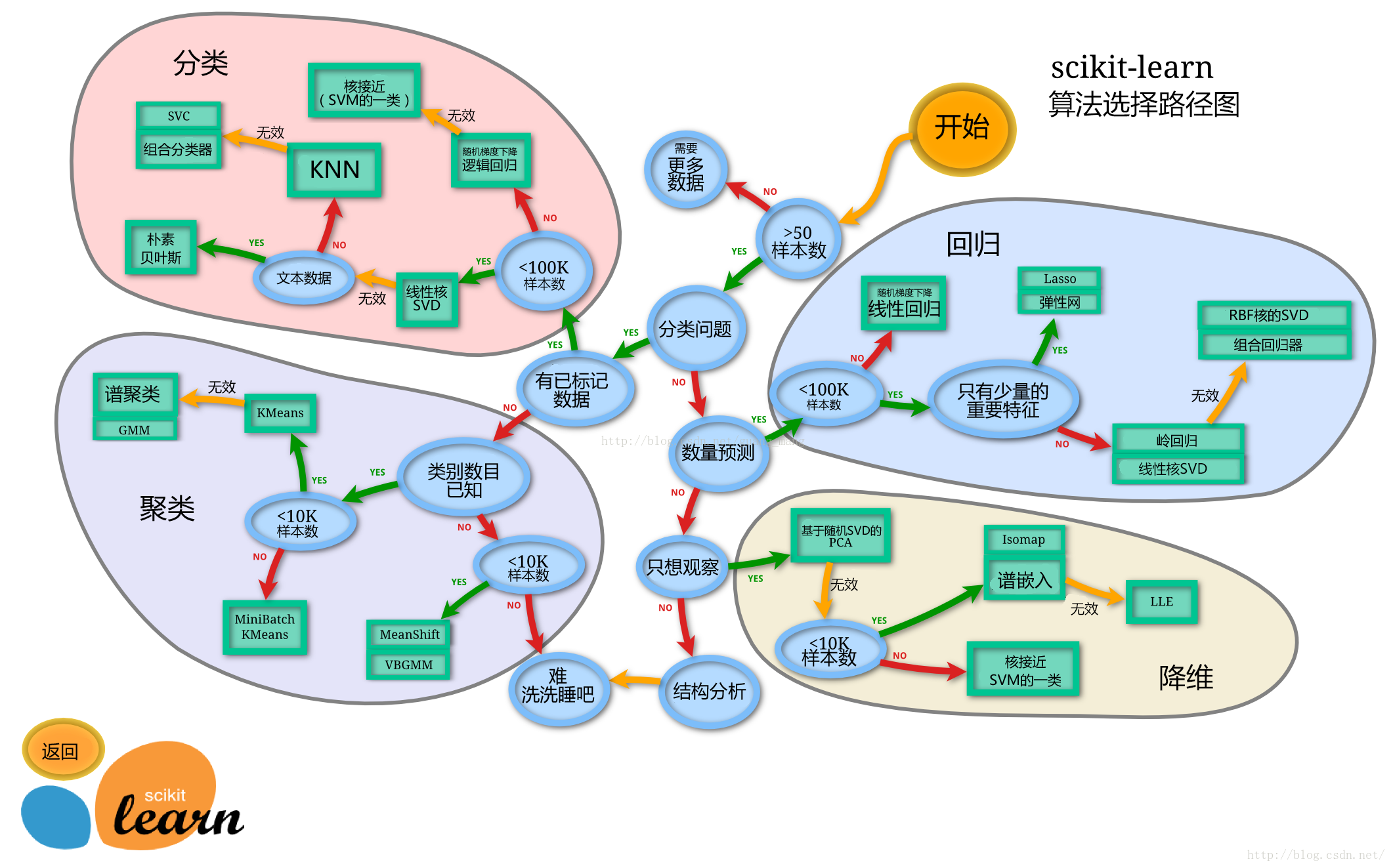
通过这几天的学习，我已经掌握了机器学习中占据大部分工作量的特征工程部分的工作内容，掌握好了这部分工作后，下面我就可以开始利用广大开源算法库来进行搭建模型，分析数据了，而算法库自然而然要想到目前最流行的scikit-learn.这个库几乎包含所有主流的机器学习算法模型，各个模型的使用教程也十分方便，话不多说，直接上图！

本次学习任务：通过之前的泰坦尼克号数据集，设计模型，完成泰坦尼克号存活预测任务。

1.1 加载库和数据集

import pandas as pd
import numpy as np
import matplotlib.pyplot as plt
import seaborn as sns
from IPython.display import Image

%matplotlib inline # 通用配置，在jupyter notebook里调用matplotlib.pyplot绘图时，使其能在控制台里面生成图像(python console)
plt.rcParams['font.sans-serif'] = ['SimHei']  # 用来正常显示中文标签
plt.rcParams['axes.unicode_minus'] = False  # 用来正常显示负号
plt.rcParams['figure.figsize'] = (10, 6)  # 设置输出图片大小

# 载入清洗之后的数据（clear_data.csv）,也可以将原始数据载入（train.csv）
df1 = pd.read_csv('clear_data.csv')
df1.head()

df1.info()

<class 'pandas.core.frame.DataFrame'>
RangeIndex: 891 entries, 0 to 890
Data columns (total 11 columns):
PassengerId    891 non-null int64
Pclass         891 non-null int64
Age            891 non-null float64
SibSp          891 non-null int64
Parch          891 non-null int64
Fare           891 non-null float64
Sex_female     891 non-null int64
Sex_male       891 non-null int64
Embarked_C     891 non-null int64
Embarked_Q     891 non-null int64
Embarked_S     891 non-null int64
dtypes: float64(2), int64(9)
memory usage: 76.6 KB

df2 = pd.read_csv('train.csv')
df2.head()

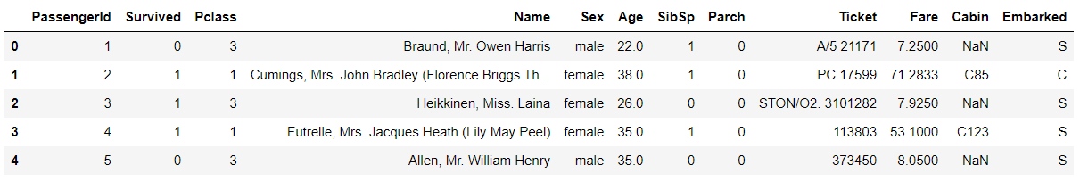
df2.info()

<class 'pandas.core.frame.DataFrame'>
RangeIndex: 891 entries, 0 to 890
Data columns (total 12 columns):
PassengerId    891 non-null int64
Survived       891 non-null int64
Pclass         891 non-null int64
Name           891 non-null object
Sex            891 non-null object
Age            714 non-null float64
SibSp          891 non-null int64
Parch          891 non-null int64
Ticket         891 non-null object
Fare           891 non-null float64
Cabin          204 non-null object
Embarked       889 non-null object
dtypes: float64(2), int64(5), object(5)
memory usage: 83.6+ KB

清洗数据集和原始数据集的对比可以看到，原始数据集有很多NA值，我们通过前面的学习方法进行了填充比如Age项，也对一些文本特征进行了独热处理，比如Sex，Embarked项。

1.2 任务一 切割训练集和测试集

• 将数据集分为自变量和因变量（X,y）
• 按比例切割训练集和测试集(一般测试集的比例有30%、25%、20%、15%和10%)
• 使用分层抽样
• 设置随机种子以便结果能复现

【思考】
1.划分数据集的方法有哪些？
sklearn.model_selection.train_test_split

train_test_split是交叉验证中常用的函数，功能是从样本中随机的按比例选取train data和testdata，形式为：
X_train,X_test, y_train, y_test =
cross_validation.train_test_split(train_data,train_target,test_size=0.4, random_state=0)

参数解释：
train_data：所要划分的样本特征集
train_target：所要划分的样本结果
test_size：样本占比，如果是整数的话就是样本的数量
random_state：是随机数的种子。
随机数种子：其实就是该组随机数的编号，在需要重复试验的时候，保证得到一组一样的随机数。比如你每次都填1，其他参数一样的情况下你得到的随机数组是一样的。但填0或不填，每次都会不一样。
随机数的产生取决于种子，随机数和种子之间的关系遵从以下两个规则：
种子不同，产生不同的随机数；种子相同，即使实例不同也产生相同的随机数。
示例

stratify: 保持分割后和分割前的数据分布相同，stratify=X 就是按照X中的比例分配，stratify=Y就是按照Y中的比例分配。
【参考】
sklearn的train_test_split()各函数参数含义解释

2. 为什么使用分层抽样，这样的好处有什么？
   分层抽样方法的优点是：样本的代表性比较好，抽样误差比较小，缺点是抽样手续比较复杂。
   分层抽样法

import sklearn
from sklearn import model_selection
y = df2['Survived'].tolist() # 标签值序列

data = df1.drop(labels = ['PassengerId', 'Embarked_C', 'Embarked_Q', 'Embarked_S'], axis=1, inplace=True) # 筛选df1中的特征，很明显，乘客编号和登船点与我们预测任务关系不大，所以筛选掉
data = np.array(df1, dtype='float') # 将DataFrame结构转换为numpy矩阵，不然无法进行训练

X = data
y_train = []
y_test = []
X_train,X_test, y_train, y_test =sklearn.model_selection.train_test_split(X,y,test_size=0.2, random_state=0)
print(X_train.shape,X_test.shape, len(y_train), len(y_test))

(712, 7) (179, 7) 712 179

【思考】：什么情况下切割数据集的时候不用进行随机选取
数据集标签值存在明显的分布规律的时候，不能进行随机选取

1.3 任务二 模型创建

• 创建基于线性模型的分类模型（逻辑回归）
• 创建基于树的分类模型（决策树、随机森林）
• 分别使用这些模型进行训练，分别的到训练集和测试集的得分
• 查看模型的参数，并更改参数值，观察模型变化

# 创建逻辑回归模型
from sklearn.linear_model import LogisticRegression
clf1 = LogisticRegression(max_iter=80, random_state=0, multi_class='auto',solver='liblinear').fit(X_train, y_train)

print(clf1.score(X_train, y_train))
print(clf1.score(X_test, y_test))

sklearn.linear_model.LogisticRegression

0.7991573033707865
0.7988826815642458

# 创建树分类模型-随机森林
from sklearn.ensemble import RandomForestClassifier
cl3 = RandomForestClassifier(max_depth=2).fit(X_train, y_train)

print(clf3.score(X_train, y_train))
print(clf3.score(X_test, y_test))

sklearn.ensemble.RandomForestClassifier

扫描二维码关注公众号，回复： 13213376 查看本文章

0.7893258426966292
0.7932960893854749

【思考】：

• 为什么线性模型可以进行分类任务，背后是怎么的数学关系
• 对于多分类问题，线性模型是怎么进行分类的

多分类问题可以看成多个二分类问题即one-vs-rest思想，比如一个三分类，可以看成是三个二分类

1.4 任务三 输出模型预测结果

• 输出模型预测分类标签
• 输出不同分类标签的预测概率

clf1.predict(X_test)

array([0, 0, 0, 1, 1, 0, 1, 1, 0, 1, 0, 1, 0, 1, 1, 1, 0, 0, 0, 0, 0, 1,
       0, 0, 1, 1, 0, 1, 1, 1, 0, 1, 0, 0, 0, 0, 0, 0, 0, 0, 0, 0, 0, 0,
       1, 0, 0, 1, 0, 0, 0, 1, 1, 0, 0, 0, 0, 0, 0, 0, 0, 1, 1, 0, 1, 0,
       1, 0, 1, 1, 1, 0, 0, 0, 0, 1, 0, 0, 0, 0, 0, 0, 1, 0, 0, 1, 1, 0,
       1, 1, 0, 0, 0, 1, 1, 0, 1, 0, 0, 1, 0, 0, 0, 0, 1, 1, 1, 0, 0, 1,
       0, 1, 0, 1, 0, 1, 1, 1, 0, 1, 0, 0, 0, 0, 0, 0, 0, 0, 0, 0, 1, 0,
       0, 1, 0, 0, 0, 0, 0, 0, 0, 1, 0, 1, 1, 1, 0, 1, 1, 0, 0, 1, 1, 0,
       1, 0, 1, 0, 1, 1, 0, 0, 1, 0, 0, 0, 0, 0, 0, 0, 0, 1, 0, 0, 1, 0,
       1, 0, 0], dtype=int64)

clf1.predict_proba(X_test)[:10]

array([[0.87857792, 0.12142208],
       [0.88111045, 0.11888955],
       [0.93438328, 0.06561672],
       [0.07879063, 0.92120937],
       [0.37103724, 0.62896276],
       [0.54809715, 0.45190285],
       [0.07713942, 0.92286058],
       [0.06265709, 0.93734291],
       [0.54550567, 0.45449433],
       [0.35127545, 0.64872455]])

二、模型搭建和评估-评估

第一部分讲述了两个分类模型，这一部分我们将学习如何判断两个模型的好坏，从哪几个方面去判断模型的性能。

import pandas as pd
import numpy as np
import seaborn as sns
import matplotlib.pyplot as plt
from IPython.display import Image
from sklearn.linear_model import LogisticRegression
from sklearn.ensemble import RandomForestClassifier

%matplotlib inline
plt.rcParams['font.sans-serif'] = ['SimHei']  # 用来正常显示中文标签
plt.rcParams['axes.unicode_minus'] = False  # 用来正常显示负号
plt.rcParams['figure.figsize'] = (10, 6)  # 设置输出图片大小

2.1 加载数据并分割测试集和训练集

from sklearn.model_selection import train_test_split
df1 = pd.read_csv('clear_data.csv')
df2 = pd.read_csv('train.csv')
X = df1
y = df2['Survived'].tolist()

# 对数据集进行切割
X_train, X_test, y_train, y_test = train_test_split(X, y, stratify=y, random_state=0)

#创建默认参数的逻辑回归模型
clf1 = LogisticRegression().fit(X_train, y_train)

2.2 模型评估

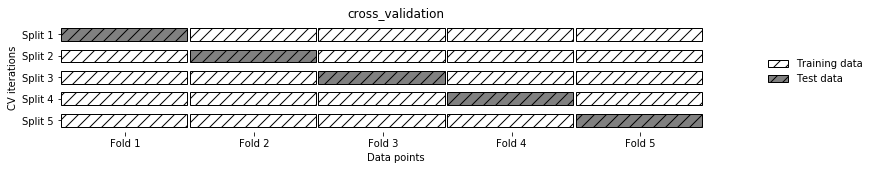
• 模型评估是为了知道模型的泛化能力。
• 交叉验证（cross-validation）是一种评估泛化性能的统计学方法，它比单次划分训练集和测试集的方法更加稳定、全面。
• 在交叉验证中，数据被多次划分，并且需要训练多个模型。
• 最常用的交叉验证是 k 折交叉验证（k-fold cross-validation），其中 k 是由用户指定的数字，通常取 5 或 10。
  【参考】：百度：交叉验证
• 准确率（precision）度量的是被预测为正例的样本中有多少是真正的正例
• 召回率（recall）度量的是正类样本中有多少被预测为正类
• f1分数是准确率与召回率的调和平均
  【参考】：吴恩达深度学习课程疑难点笔记系列-结构化机器学习项目-第1周&第2周

2.2.1 交叉验证

• 用10折交叉验证来评估之前的逻辑回归模型
• 计算交叉验证精度的平均值
  

from sklearn.model_selection import cross_val_score
clf1 = LogisticRegression(C=100)
scores = cross_val_score(lr, X_train, y_train, cv=10)

# K折交叉验证分数
scores

array([0.85074627, 0.74626866, 0.74626866, 0.80597015, 0.88059701,
       0.8358209 , 0.76119403, 0.8358209 , 0.74242424, 0.75757576])

# 平均交叉验证分数
print("Average cross-validation score: {:.2f}".format(scores.mean()))

Average cross-validation score: 0.80

【思考】K折越多的情况下会带来什么样的影响？
增大k值，在每次迭代过程中将会有更多的数据用于模型训练，能够得到最小偏差，同时算法时间延长。且训练块间高度相似，导致评价结果方差较高。

2.2.2 混淆矩阵

• 计算二分类问题的混淆矩阵
• 计算精确率、召回率以及f1分数

混淆矩阵也称误差矩阵，是表示精度评价的一种标准格式，用n行n列的矩阵形式来表示。

参考：分类器模型评估指标之混淆矩阵（二分类/多分类）
吴恩达深度学习课程疑难点笔记系列-结构化机器学习项目-第1周&第2周

from sklearn.metrics import confusion_matrix
pred = clf1.predict(X_train) # 模型预测结果
confusion_matrix(y_train, pred) # 混淆矩阵

array([[354, 58],
[ 83, 173]])

from sklearn.metrics import classification_report
print(classification_report(y_train, pred)

precision recall f1-score support

       0       0.81      0.86      0.83       412
       1       0.75      0.68      0.71       256

accuracy                           0.79       668

macro avg 0.78 0.77 0.77 668
weighted avg 0.79 0.79 0.79 668

【参考】：sklearn.metrics.classification_report

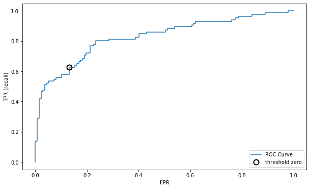
2.2.3 ROC曲线

【官方教程】：roc_curve

from sklearn.metrics import roc_curve

fpr, tpr, thresholds = roc_curve(y_test, cf1.decision_function(X_test))
plt.plot(fpr, tpr, label="ROC Curve")
plt.xlabel("FPR")
plt.ylabel("TPR (recall)")
# 找到最接近于0的阈值
close_zero = np.argmin(np.abs(thresholds))
plt.plot(fpr[close_zero], tpr[close_zero], 'o', markersize=10, label="threshold zero", fillstyle="none", c='k', mew=2)
plt.legend(loc=4)

多分类模型的ROC曲线绘制：