【数据分析入门】动手学数据分析 Task5 模型建立和评估

Task5： 模型建立和评估

通过导入kaggle上泰坦尼克的数据集，实战数据分析全流程

项目地址: 动手学数据分析

1. 第三章 模型搭建和评估–建模

经过前面的两章的知识点的学习，我可以对数数据的本身进行处理，比如数据本身的增删查补，还可以做必要的清洗工作。那么下面我们就要开始使用我们前面处理好的数据了。这一章我们要做的就是使用数据，我们做数据分析的目的也就是，运用我们的数据以及结合我的业务来得到某些我们需要知道的结果。那么分析的第一步就是建模，搭建一个预测模型或者其他模型；我们从这个模型的到结果之后，我们要分析我的模型是不是足够的可靠，那我就需要评估这个模型。今天我们学习建模，下一节我们学习评估。

我们拥有的泰坦尼克号的数据集，那么我们这次的目的就是，完成泰坦尼克号存活预测这个任务。

import pandas as pd
import numpy as np
import matplotlib.pyplot as plt
import seaborn as sns
from IPython.display import Image

%matplotlib inline

plt.rcParams['font.sans-serif'] = ['SimHei']  # 用来正常显示中文标签
plt.rcParams['axes.unicode_minus'] = False  # 用来正常显示负号
plt.rcParams['figure.figsize'] = (10, 6)  # 设置输出图片大小

from IPython.core.interactiveshell import InteractiveShell
InteractiveShell.ast_node_interactivity = "all"

载入这些库，如果缺少某些库，请安装他们

【思考】这些库的作用是什么呢？你需要查一查

【思考回答】这些库的作用是什么呢？

numpy 科学计算库
pandas 基于numpy的数据操作库
matplotlib python基础绘图库
seaborn 基于matplotlib的绘图库

%matplotlib inline

载入我们提供清洗之后的数据(clear_data.csv)，大家也将原始数据载入（train.csv），说说他们有什么不同

#写入代码
df = pd.read_csv("clear_data.csv")
df.shape
df.head()

(891, 11)

	PassengerId	Pclass	Age	SibSp	Parch	Fare	Sex_female	Sex_male	Embarked_C	Embarked_Q	Embarked_S
0	0	3	22.0	1	0	7.2500	0	1	0	0	1
1	1	1	38.0	1	0	71.2833	1	0	1	0	0
2	2	3	26.0	0	0	7.9250	1	0	0	0	1
3	3	1	35.0	1	0	53.1000	1	0	0	0	1
4	4	3	35.0	0	0	8.0500	0	1	0	0	1

df.isnull().sum()

PassengerId    0
Pclass         0
Age            0
SibSp          0
Parch          0
Fare           0
Sex_female     0
Sex_male       0
Embarked_C     0
Embarked_Q     0
Embarked_S     0
dtype: int64

#写入代码
df_origin = pd.read_csv("train.csv")
df_origin.shape
df_origin.head()

 (891, 12)

	PassengerId	Survived	Pclass	Name	Sex	Age	SibSp	Parch	Ticket	Fare	Cabin	Embarked
0	1	0	3	Braund, Mr. Owen Harris	male	22.0	1	0	A/5 21171	7.2500	NaN	S
1	2	1	1	Cumings, Mrs. John Bradley (Florence Briggs Th...	female	38.0	1	0	PC 17599	71.2833	C85	C
2	3	1	3	Heikkinen, Miss. Laina	female	26.0	0	0	STON/O2. 3101282	7.9250	NaN	S
3	4	1	1	Futrelle, Mrs. Jacques Heath (Lily May Peel)	female	35.0	1	0	113803	53.1000	C123	S
4	5	0	3	Allen, Mr. William Henry	male	35.0	0	0	373450	8.0500	NaN	S

【思考回答】二者不同之处

1. 将Survived列取出作为预测结果列
2. 将Sex和Embarked列透视
3. 将Ticket,Name和Cabin取出

模型搭建

• 处理完前面的数据我们就得到建模数据，下一步是选择合适模型
• 在进行模型选择之前我们需要先知道数据集最终是进行监督学习还是无监督学习
• 模型的选择一方面是通过我们的任务来决定的。
• 除了根据我们任务来选择模型外，还可以根据数据样本量以及特征的稀疏性来决定
• 刚开始我们总是先尝试使用一个基本的模型来作为其baseline，进而再训练其他模型做对比，最终选择泛化能力或性能比较好的模型

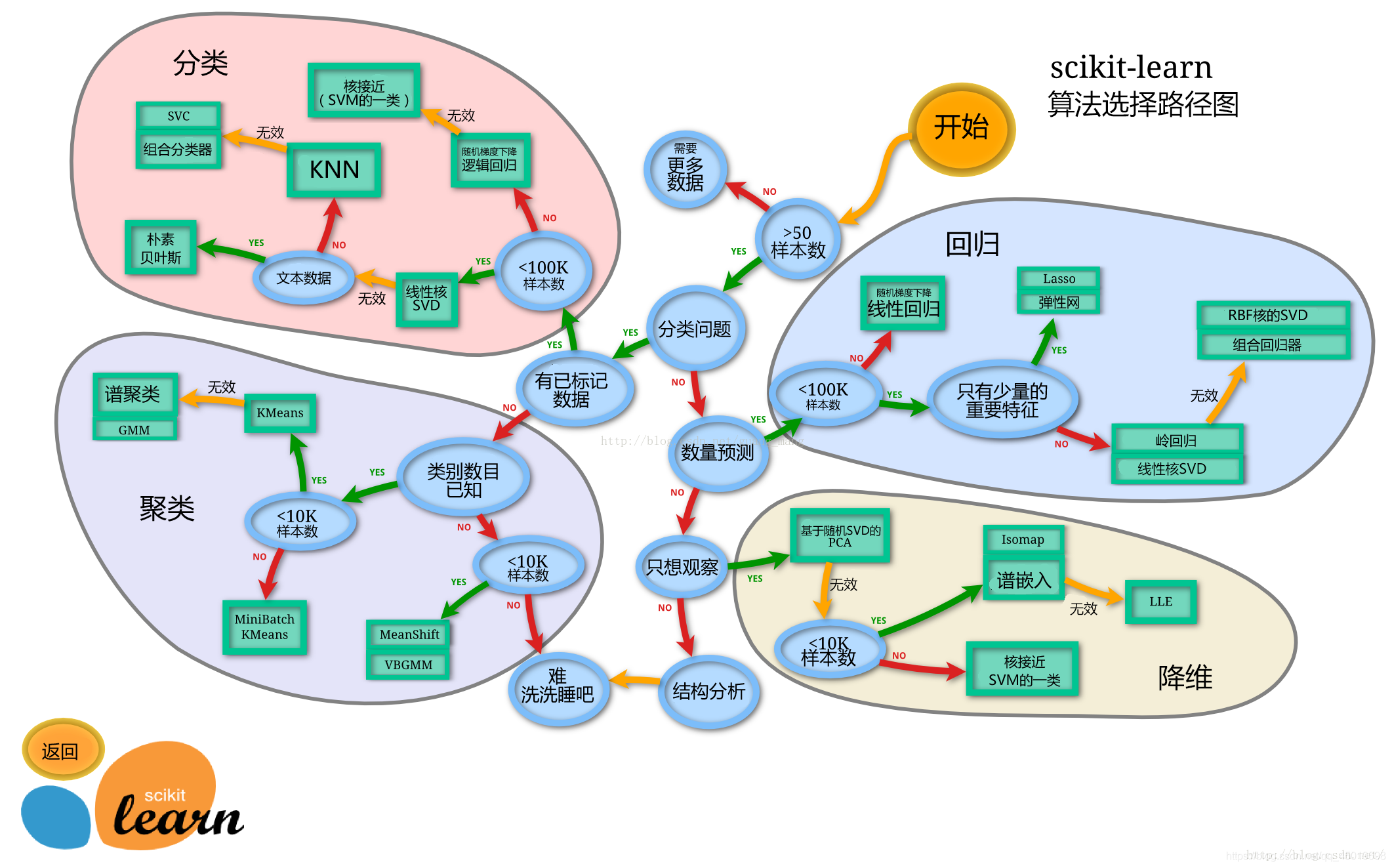
我们这里使用一个机器学习最常用的一个库（sklearn）来完成我们的模型的搭建

下面给出sklearn的算法选择路径，供大家参考

# sklearn模型算法选择路径图
Image('sklearn.png')

【思考回答】数据集哪些差异会导致模型在拟合数据是发生变化

数据集的大小和数据集的维度

任务一：切割训练集和测试集

这里使用留出法划分数据集

• 将数据集分为自变量和因变量
• 按比例切割训练集和测试集(一般测试集的比例有30%、25%、20%、15%和10%)
• 使用分层抽样
• 设置随机种子以便结果能复现

【思考】

• 划分数据集的方法有哪些？
• 为什么使用分层抽样，这样的好处有什么？

【思考回答】划分数据集的方法有哪些？

1. 留出法。 将数据集D划分为两个互斥的集合，其中一个集合作为训练集S，另一个集合作为测试集T，即D=S∪T，S∩T=∅。在S上训练出模型后，用T来评估其误差
2. 交叉验证法。 将数据集D划分为 k 个大小相似的互斥子集，即D=D1∪D2∪⋯∪Dk，Di∩Dj=∅（i≠j）。每个子集都要尽可能保持数据分布的一致性，即从D中通过分层采样得到。然后用 (k−1) 个子集的并集作为训练集，余下的子集作为测试集。这样就可以获得 k 组训练/测试集，从而可以进行 k 次训练和测试，最终返回的是 k 个测试结果的均值。
3. 自助法。

样本的代表性比较好，抽样误差比较小

任务提示

• 切割数据集是为了后续能评估模型泛化能力
• sklearn中切割数据集的方法为train_test_split
• 查看函数文档可以在jupyter noteboo里面使用train_test_split?后回车即可看到
• 分层和随机种子在参数里寻找

要从clear_data.csv和train.csv中提取train_test_split()所需的参数

#写入代码
from sklearn.model_selection import train_test_split
df_x = df.copy()
df_origin_y = df_origin.copy()

#写入代码
X = df_x
y = df_origin_y['Survived']

#写入代码

X_train, X_test, y_train, y_test = train_test_split(X,y,stratify=y,random_state=0)

#写入代码
X_train.shape
X_test.shape

(668, 11)


(223, 11)

任务二：模型创建

• 创建基于线性模型的分类模型（逻辑回归）
• 创建基于树的分类模型（决策树、随机森林）
• 分别使用这些模型进行训练，分别的到训练集和测试集的得分
• 查看模型的参数，并更改参数值，观察模型变化

提示

• 逻辑回归不是回归模型而是分类模型，不要与LinearRegression混淆
• 随机森林其实是决策树集成为了降低决策树过拟合的情况
• 线性模型所在的模块为sklearn.linear_model
• 树模型所在的模块为sklearn.ensemble

#写入代码
# 线性回归
from sklearn.linear_model import LogisticRegression
# 随机森林
from sklearn.ensemble import RandomForestClassifier

#写入代码
lr = LogisticRegression()
lr.fit(X_train, y_train)

E:\Anaconda\lib\site-packages\sklearn\linear_model\_logistic.py:940: ConvergenceWarning: lbfgs failed to converge (status=1):
STOP: TOTAL NO. of ITERATIONS REACHED LIMIT.

Increase the number of iterations (max_iter) or scale the data as shown in:
    https://scikit-learn.org/stable/modules/preprocessing.html
Please also refer to the documentation for alternative solver options:
    https://scikit-learn.org/stable/modules/linear_model.html#logistic-regression
  extra_warning_msg=_LOGISTIC_SOLVER_CONVERGENCE_MSG)





LogisticRegression(C=1.0, class_weight=None, dual=False, fit_intercept=True,
                   intercept_scaling=1, l1_ratio=None, max_iter=100,
                   multi_class='auto', n_jobs=None, penalty='l2',
                   random_state=None, solver='lbfgs', tol=0.0001, verbose=0,
                   warm_start=False)

#写入代码
print("Logistic train score:{:.2f}".format(lr.score(X_train, y_train)))
print("Logistic test score:{:.2f}".format(lr.score(X_test, y_test)))

Logistic train score:0.80
Logistic test score:0.79

#写入代码
lr_C = LogisticRegression(C=200)
lr_C.fit(X_train, y_train)

E:\Anaconda\lib\site-packages\sklearn\linear_model\_logistic.py:940: ConvergenceWarning: lbfgs failed to converge (status=1):
STOP: TOTAL NO. of ITERATIONS REACHED LIMIT.

Increase the number of iterations (max_iter) or scale the data as shown in:
    https://scikit-learn.org/stable/modules/preprocessing.html
Please also refer to the documentation for alternative solver options:
    https://scikit-learn.org/stable/modules/linear_model.html#logistic-regression
  extra_warning_msg=_LOGISTIC_SOLVER_CONVERGENCE_MSG)





LogisticRegression(C=200, class_weight=None, dual=False, fit_intercept=True,
                   intercept_scaling=1, l1_ratio=None, max_iter=100,
                   multi_class='auto', n_jobs=None, penalty='l2',
                   random_state=None, solver='lbfgs', tol=0.0001, verbose=0,
                   warm_start=False)

print("Logistic train score:{:.2f}".format(lr_C.score(X_train, y_train)))
print("Logistic test score:{:.2f}".format(lr_C.score(X_test, y_test)))

Logistic train score:0.80
Logistic test score:0.78

Rf = RandomForestClassifier()
Rf.fit(X_train, y_train)

RandomForestClassifier(bootstrap=True, ccp_alpha=0.0, class_weight=None,
                       criterion='gini', max_depth=None, max_features='auto',
                       max_leaf_nodes=None, max_samples=None,
                       min_impurity_decrease=0.0, min_impurity_split=None,
                       min_samples_leaf=1, min_samples_split=2,
                       min_weight_fraction_leaf=0.0, n_estimators=100,
                       n_jobs=None, oob_score=False, random_state=None,
                       verbose=0, warm_start=False)

print("RandomForestRegressor set score: {:.2f}".format(Rf.score(X_train, y_train)))
print("RandomForestRegressor set score: {:.2f}".format(Rf.score(X_test, y_test)))

RandomForestRegressor set score: 1.00
RandomForestRegressor set score: 0.82

Rf = RandomForestClassifier(max_depth=10, random_state=0)
Rf.fit(X_train, y_train)

RandomForestClassifier(bootstrap=True, ccp_alpha=0.0, class_weight=None,
                       criterion='gini', max_depth=10, max_features='auto',
                       max_leaf_nodes=None, max_samples=None,
                       min_impurity_decrease=0.0, min_impurity_split=None,
                       min_samples_leaf=1, min_samples_split=2,
                       min_weight_fraction_leaf=0.0, n_estimators=100,
                       n_jobs=None, oob_score=False, random_state=0, verbose=0,
                       warm_start=False)

print("RandomForestRegressor set score: {:.2f}".format(Rf.score(X_train, y_train)))
print("RandomForestRegressor set score: {:.2f}".format(Rf.score(X_test, y_test)))

RandomForestRegressor set score: 0.97
RandomForestRegressor set score: 0.81

# 调整参数后的随机森林分类模型
Rf2 = RandomForestClassifier(n_estimators=100, max_depth=10)
Rf2.fit(X_train, y_train)

RandomForestClassifier(bootstrap=True, ccp_alpha=0.0, class_weight=None,
                       criterion='gini', max_depth=10, max_features='auto',
                       max_leaf_nodes=None, max_samples=None,
                       min_impurity_decrease=0.0, min_impurity_split=None,
                       min_samples_leaf=1, min_samples_split=2,
                       min_weight_fraction_leaf=0.0, n_estimators=100,
                       n_jobs=None, oob_score=False, random_state=None,
                       verbose=0, warm_start=False)

print("RandomForestRegressor set score: {:.2f}".format(Rf2.score(X_train, y_train)))
print("RandomForestRegressor set score: {:.2f}".format(Rf2.score(X_test, y_test)))

RandomForestRegressor set score: 0.97
RandomForestRegressor set score: 0.82

【思考】为什么线性模型可以进行分类任务，背后是怎么的数学关系

• 为什么线性模型可以进行分类任务，背后是怎么的数学关系
• 对于多分类问题，线性模型是怎么进行分类的

任务三：输出模型预测结果

• 输出模型预测分类标签
• 输出不同分类标签的预测概率

任务提示

• 一般监督模型在sklearn里面有个predict能输出预测标签，predict_proba则可以输出标签概率

#写入代码
pred = lr.predict(X_train)
pred[:10]

array([0, 1, 1, 1, 0, 0, 1, 0, 1, 1], dtype=int64)

#写入代码


pred_proba = lr.predict_proba(X_train)
pred_proba[:10]

array([[0.60729586, 0.39270414],
       [0.18238096, 0.81761904],
       [0.42258598, 0.57741402],
       [0.19331014, 0.80668986],
       [0.8793502 , 0.1206498 ],
       [0.91331757, 0.08668243],
       [0.13394337, 0.86605663],
       [0.90560106, 0.09439894],
       [0.05273676, 0.94726324],
       [0.10973509, 0.89026491]])

#写入代码
pred = Rf.predict(X_train)
pred[:10]

array([0, 1, 0, 1, 0, 0, 1, 1, 1, 1], dtype=int64)

#写入代码

pred_proda = Rf.predict_proba(X_train)
pred_proda[:10]

array([[5.78762372e-01, 4.21237628e-01],
       [1.34703717e-02, 9.86529628e-01],
       [9.62833333e-01, 3.71666667e-02],
       [1.37413792e-01, 8.62586208e-01],
       [9.64440891e-01, 3.55591094e-02],
       [9.40065876e-01, 5.99341240e-02],
       [1.69033973e-02, 9.83096603e-01],
       [2.11054122e-01, 7.88945878e-01],
       [6.66666667e-04, 9.99333333e-01],
       [4.06666667e-02, 9.59333333e-01]])

2. 第三章 模型搭建和评估-评估

根据之前的模型的建模，我们知道如何运用sklearn这个库来完成建模，以及我们知道了的数据集的划分等等操作。那么一个模型我们怎么知道它好不好用呢？以至于我们能不能放心的使用模型给我的结果呢？那么今天的学习的评估，就会很有帮助。

加载下面的库

import pandas as pd
import numpy as np
import seaborn as sns
import matplotlib.pyplot as plt
from IPython.display import Image
from sklearn.linear_model import LogisticRegression
from sklearn.ensemble import RandomForestClassifier

%matplotlib inline

plt.rcParams['font.sans-serif'] = ['SimHei']  # 用来正常显示中文标签
plt.rcParams['axes.unicode_minus'] = False  # 用来正常显示负号
plt.rcParams['figure.figsize'] = (10, 6)  # 设置输出图片大小

from IPython.core.interactiveshell import InteractiveShell
InteractiveShell.ast_node_interactivity = "all"

任务：加载数据并分割测试集和训练集

from sklearn.model_selection import train_test_split

#写入代码
df = pd.read_csv('clear_data.csv')
train = pd.read_csv('train.csv')
X = df
y = train['Survived']

#写入代码
X_train, X_test, y_train, y_test = train_test_split(X, y, stratify=y, random_state=0)

#写入代码
lr = LogisticRegression()
lr.fit(X_train, y_train)

E:\Anaconda\lib\site-packages\sklearn\linear_model\_logistic.py:940: ConvergenceWarning: lbfgs failed to converge (status=1):
STOP: TOTAL NO. of ITERATIONS REACHED LIMIT.

Increase the number of iterations (max_iter) or scale the data as shown in:
    https://scikit-learn.org/stable/modules/preprocessing.html
Please also refer to the documentation for alternative solver options:
    https://scikit-learn.org/stable/modules/linear_model.html#logistic-regression
  extra_warning_msg=_LOGISTIC_SOLVER_CONVERGENCE_MSG)





LogisticRegression(C=1.0, class_weight=None, dual=False, fit_intercept=True,
                   intercept_scaling=1, l1_ratio=None, max_iter=100,
                   multi_class='auto', n_jobs=None, penalty='l2',
                   random_state=None, solver='lbfgs', tol=0.0001, verbose=0,
                   warm_start=False)

模型评估

• 模型评估是为了知道模型的泛化能力。
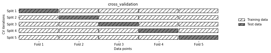
• 交叉验证（cross-validation）是一种评估泛化性能的统计学方法，它比单次划分训练集和测试集的方法更加稳定、全面。
• 在交叉验证中，数据被多次划分，并且需要训练多个模型。
• 最常用的交叉验证是 k 折交叉验证（k-fold cross-validation），其中 k 是由用户指定的数字，通常取 5 或 10。
• 准确率（precision）度量的是被预测为正例的样本中有多少是真正的正例
• 召回率（recall）度量的是正类样本中有多少被预测为正类
• f-分数是准确率与召回率的调和平均

【思考回答】：将上面的概念进一步的理解，大家可以做一下总结

在使用训练集对参数进行训练的时候，经常会发现人们通常会将一整个训练集分为三个部分（比如mnist手写训练集）。一般分为：训练集（train_set），评估集（valid_set），测试集（test_set）这三个部分。这其实是为了保证训练效果而特意设置的。其中测试集很好理解，其实就是完全不参与训练的数据，仅仅用来观测测试效果的数据。

因为在实际的训练中，训练的结果对于训练集的拟合程度通常还是挺好的（初始条件敏感），但是对于训练集之外的数据的拟合程度通常就不那么令人满意了。因此我们通常并不会把所有的数据集都拿来训练，而是分出一部分来（这一部分不参加训练）对训练集生成的参数进行测试，相对客观的判断这些参数对训练集之外的数据的符合程度。这种思想就称为交叉验证（Cross Validation）

任务一：交叉验证

• 用10折交叉验证来评估之前的逻辑回归模型
• 计算交叉验证精度的平均值

#提示：交叉验证
Image('Snipaste_2020-01-05_16-37-56.png')

任务提示

• 交叉验证在sklearn中的模块为sklearn.model_selection

#写入代码
from sklearn.model_selection import cross_val_score

#写入代码
# 定义模型
lr = LogisticRegression()
# cross_val_score(estimator, X, y=None, *, groups=None, scoring=None, cv=None, n_jobs=None, verbose=0, fit_params=None, pre_dispatch='2*n_jobs', error_score=nan)
# estimator 分类器 用于训练
# X : 被训练的数据集
# y : 预测的目标变量
# scoring: 评分调用方法
# cv ： 确定分折数
# n_jobs : 用于进行计算的CPU数量
scores = cross_val_score(lr, X_train, y_train, cv=10)

#写入代码
scores
scores.mean()

array([0.85074627, 0.76119403, 0.76119403, 0.80597015, 0.88059701,
       0.85074627, 0.76119403, 0.85074627, 0.75757576, 0.72727273])






0.8007236544549977

#写入代码
# 平均交叉验证分数
print("Average cross-validation score: {:.2f}".format(scores.mean()))

Average cross-validation score: 0.80

【思考回答】k折越多的情况下会带来什么样的影响？

当数据量较大时，使用较大K值的计算开销远远超过了我们的承受能力，需要谨慎对待

当模型稳定性较低时，增大K的取值可以给出更好的结果。

任务二：混淆矩阵

• 计算二分类问题的混淆矩阵
• 计算精确率、召回率以及f-分数

【思考回答】什么是二分类问题的混淆矩阵，理解这个概念，知道它主要是运算到什么任务中的

混淆矩阵是对分类问题的预测结果的总结。使用计数值汇总正确和不正确预测的数量，并按每个类进行细分，这是混淆矩阵的关键所在。混淆矩阵显示了分类模型的在进行预测时会对哪一部分产生混淆。

#提示：混淆矩阵
Image('Snipaste_2020-01-05_16-38-26.png')

#提示：准确率 (Accuracy),精确度（Precision）,Recall,f-分数计算方法
Image('Snipaste_2020-01-05_16-39-27.png')

提示

• 混淆矩阵的方法在sklearn中的sklearn.metrics模块
• 混淆矩阵需要输入真实标签和预测标签
• 精确率、召回率以及f-分数可使用classification_report模块

#写入代码
from sklearn.metrics import confusion_matrix

#写入代码
lr = LogisticRegression(C=100)
lr.fit(X_train, y_train)

LogisticRegression(C=100, class_weight=None, dual=False, fit_intercept=True,
                   intercept_scaling=1, l1_ratio=None, max_iter=100,
                   multi_class='auto', n_jobs=None, penalty='l2',
                   random_state=None, solver='lbfgs', tol=0.0001, verbose=0,
                   warm_start=False)

#写入代码
pred = lr.predict(X_train)

#写入代码
confusion_matrix(y_train, pred)

array([[354,  58],
       [ 83, 173]], dtype=int64)

任务三：ROC曲线

• 绘制ROC曲线

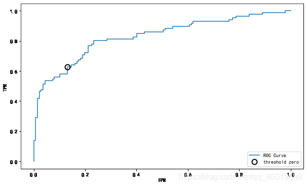
【思考回答】什么是ROC曲线，ROC曲线的存在是为了解决什么问题？

“ROC 曲线（接收者操作特征曲线）是一种显示分类模型在所有分类阈值下的效果的图表。"
平面的横坐标是false positive rate(FPR)，纵坐标是true positive rate(TPR)

TPR = TP / (TP + FN) (也就是Recall)

FPR = FP / (FP + TN)

当测试集中的正负样本的分布变化的时候，ROC曲线能够保持不变。在实际的数据集中经常会出现类不平衡（class imbalance）现象，即负样本比正样本多很多（或者相反），而且测试数据中的正负样本的分布也可能随着时间变化。

提示

• ROC曲线在sklearn中的模块为sklearn.metrics
• ROC曲线下面所包围的面积越大越好

#写入代码
from sklearn.metrics import roc_curve

#写入代码
fpr, tpr, thresholds = roc_curve(y_test, lr.decision_function(X_test))
plt.plot(fpr, tpr, label="ROC Curve")
plt.xlabel("FPR")
plt.ylabel("TPR ")
close_zero = np.argmin(np.abs(thresholds))
plt.plot(fpr[close_zero], tpr[close_zero], 'o', markersize=10, label="threshold zero", fillstyle="none", c="k", mew=2)
plt.legend(loc=4)

[<matplotlib.lines.Line2D at 0x20570d49780>]

Text(0.5, 0, 'FPR')

Text(0, 0.5, 'TPR ')

[<matplotlib.lines.Line2D at 0x20570d49b70>]

<matplotlib.legend.Legend at 0x20570d49e48>

【思考回答】对于多分类问题如何绘制ROC曲线

①方法一：每种类别下，都可以得到m个测试样本为该类别的概率（矩阵P中的列）。所以，根据概率矩阵P和标签矩阵L中对应的每一列，可以计算出各个阈值下的假正例率（FPR）和真正例率（TPR），从而绘制出一条ROC曲线。这样总共可以绘制出n条ROC曲线。最后对n条ROC曲线取平均，即可得到最终的ROC曲线。

②方法二：
首先，对于一个测试样本：1）标签只由0和1组成，1的位置表明了它的类别（可对应二分类问题中的‘’正’’），0就表示其他类别（‘’负‘’）；2）要是分类器对该测试样本分类正确，则该样本标签中1对应的位置在概率矩阵P中的值是大于0对应的位置的概率值的。基于这两点，将标签矩阵L和概率矩阵P分别按行展开，转置后形成两列，这就得到了一个二分类的结果。所以，此方法经过计算后可以直接得到最终的ROC曲线。

import numpy as np
import matplotlib.pyplot as plt
from itertools import cycle
from sklearn import svm, datasets
from sklearn.metrics import roc_curve, auc
from sklearn.model_selection import train_test_split
from sklearn.preprocessing import label_binarize
from sklearn.multiclass import OneVsRestClassifier
from scipy import interp

# 加载数据
iris = datasets.load_iris()
X = iris.data
y = iris.target
# 将标签二值化
y = label_binarize(y, classes=[0, 1, 2])
# 设置种类
n_classes = y.shape[1]

# 训练模型并预测
random_state = np.random.RandomState(0)
n_samples, n_features = X.shape

# shuffle and split training and test sets
X_train, X_test, y_train, y_test = train_test_split(X, y, test_size=.5,random_state=0)

# Learn to predict each class against the other
classifier = OneVsRestClassifier(svm.SVC(kernel='linear', probability=True,
                                 random_state=random_state))
y_score = classifier.fit(X_train, y_train).decision_function(X_test)

# 计算每一类的ROC
fpr = dict()
tpr = dict()
roc_auc = dict()
for i in range(n_classes):
    fpr[i], tpr[i], _ = roc_curve(y_test[:, i], y_score[:, i])
    roc_auc[i] = auc(fpr[i], tpr[i])

# Compute micro-average ROC curve and ROC area（方法二）
fpr["micro"], tpr["micro"], _ = roc_curve(y_test.ravel(), y_score.ravel())
roc_auc["micro"] = auc(fpr["micro"], tpr["micro"])

# Compute macro-average ROC curve and ROC area（方法一）
# First aggregate all false positive rates
all_fpr = np.unique(np.concatenate([fpr[i] for i in range(n_classes)]))
# Then interpolate all ROC curves at this points
mean_tpr = np.zeros_like(all_fpr)
for i in range(n_classes):
    mean_tpr += interp(all_fpr, fpr[i], tpr[i])
# Finally average it and compute AUC
mean_tpr /= n_classes
fpr["macro"] = all_fpr
tpr["macro"] = mean_tpr
roc_auc["macro"] = auc(fpr["macro"], tpr["macro"])

# Plot all ROC curves
lw=2
plt.figure()
plt.plot(fpr["micro"], tpr["micro"],
         label='micro-average ROC curve (area = {0:0.2f})'
               ''.format(roc_auc["micro"]),
         color='deeppink', linestyle=':', linewidth=4)

plt.plot(fpr["macro"], tpr["macro"],
         label='macro-average ROC curve (area = {0:0.2f})'
               ''.format(roc_auc["macro"]),
         color='navy', linestyle=':', linewidth=4)

colors = cycle(['aqua', 'darkorange', 'cornflowerblue'])
for i, color in zip(range(n_classes), colors):
    plt.plot(fpr[i], tpr[i], color=color, lw=lw,
             label='ROC curve of class {0} (area = {1:0.2f})'
             ''.format(i, roc_auc[i]))

plt.plot([0, 1], [0, 1], 'k--', lw=lw)
plt.xlim([0.0, 1.0])
plt.ylim([0.0, 1.05])
plt.xlabel('False Positive Rate')
plt.ylabel('True Positive Rate')
plt.title('Some extension of Receiver operating characteristic to multi-class')
plt.legend(loc="lower right")
plt.show()

<Figure size 720x432 with 0 Axes>
[<matplotlib.lines.Line2D at 0x20570f6a5c0>]
[<matplotlib.lines.Line2D at 0x20570f44518>]

[<matplotlib.lines.Line2D at 0x2056ebf85c0>]

[<matplotlib.lines.Line2D at 0x20570f6ac50>]

[<matplotlib.lines.Line2D at 0x20570f6afd0>]

[<matplotlib.lines.Line2D at 0x20570f77668>]

(0.0, 1.0)

(0.0, 1.05)

Text(0.5, 0, 'False Positive Rate')

Text(0, 0.5, 'True Positive Rate')

Text(0.5, 1.0, 'Some extension of Receiver operating characteristic to multi-class')

<matplotlib.legend.Legend at 0x20570f52dd8>