【论文阅读】A Gentle Introduction to Graph Neural Networks [图神经网络入门]（4）

The challenges of using graphs in machine learning
图在机器学习中的应用挑战

So, how do we go about solving these different graph tasks with neural networks? The first step is to think about how we will represent graphs to be compatible with neural networks.
那么，我们如何用神经网络来解决这些不同的图的预测任务呢?第一步是考虑如何表示与神经网络兼容的图。

Machine learning models typically take rectangular or grid-like arrays as input. So, it’s not immediately intuitive how to represent them in a format that is compatible with deep learning. Graphs have up to four types of information that we will potentially want to use to make predictions: nodes, edges, global-context and connectivity. The first three are relatively straightforward: for example, with nodes we can form a node feature matrix $N$ by assigning each node an index $i$ and storing the feature for $nod{e}_i$ in $N$. While these matrices have a variable number of examples, they can be processed without any special techniques.
机器学习模型通常采用矩形或网格状array作为输入。因此，如何用一种与深度学习兼容的格式来表示它们并不是一种直观的方法。图有多达四种类型的信息，我们可能希望使用它们来进行预测:节点、边、全局上下文和连通性。前三个相对简单: 例如，对于节点，我们可以为每个节点分配一个索引$i$，并将$nod{e}_i$的特征存储在$N$中，从而形成一个节点特征矩阵$N$。虽然这些矩阵的示例数量是可变的，但它们无需任何特殊技术就可以处理。

However, representing a graph’s connectivity is more complicated. Perhaps the most obvious choice would be to use an adjacency matrix, since this is easily tensorisable. However, this representation has a few drawbacks. From the example dataset table, we see the number of nodes in a graph can be on the order of millions, and the number of edges per node can be highly variable. Often, this leads to very sparse adjacency matrices, which are space-inefficient.
然而，表示图的连通性要复杂得多。也许最明智的选择是使用邻接矩阵来表示图的连通性，因为它很容易被表示为张量。但是，这种表示方式有一些缺点。从示例数据集表中，我们可以看到图中的节点数可以达到数百万的量级，每个节点的边数可以是高度可变的。这通常会导致非常稀疏的邻接矩阵，这使得空间的存储效率很低。

Another problem is that there are many adjacency matrices that can encode the same connectivity, and there is no guarantee that these different matrices would produce the same result in a deep neural network (that is to say, they are not permutation invariant).
另一个问题是，有许多邻接矩阵在编码后具有相同的连通性，并且不能保证这些不同的矩阵会在深度神经网络中产生相同的结果(也就是说，它们不是置换不变的)。

Learning permutation invariant operations is an area of recent research.[16] [17]
学习置换不变运算是最近研究的一个领域。[16] [17]

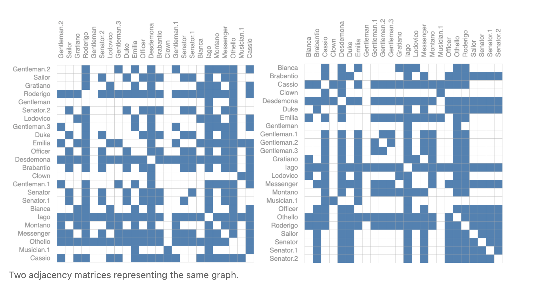
For example, the Othello graph from before can be described equivalently with these two adjacency matrices. It can also be described with every other possible permutation of the nodes.
例如，前面的奥赛罗图可以用以下这两个邻接矩阵等价地描述。它也可以用所有其他可能的节点排列来描述。

表示同一个图的两个邻接矩阵

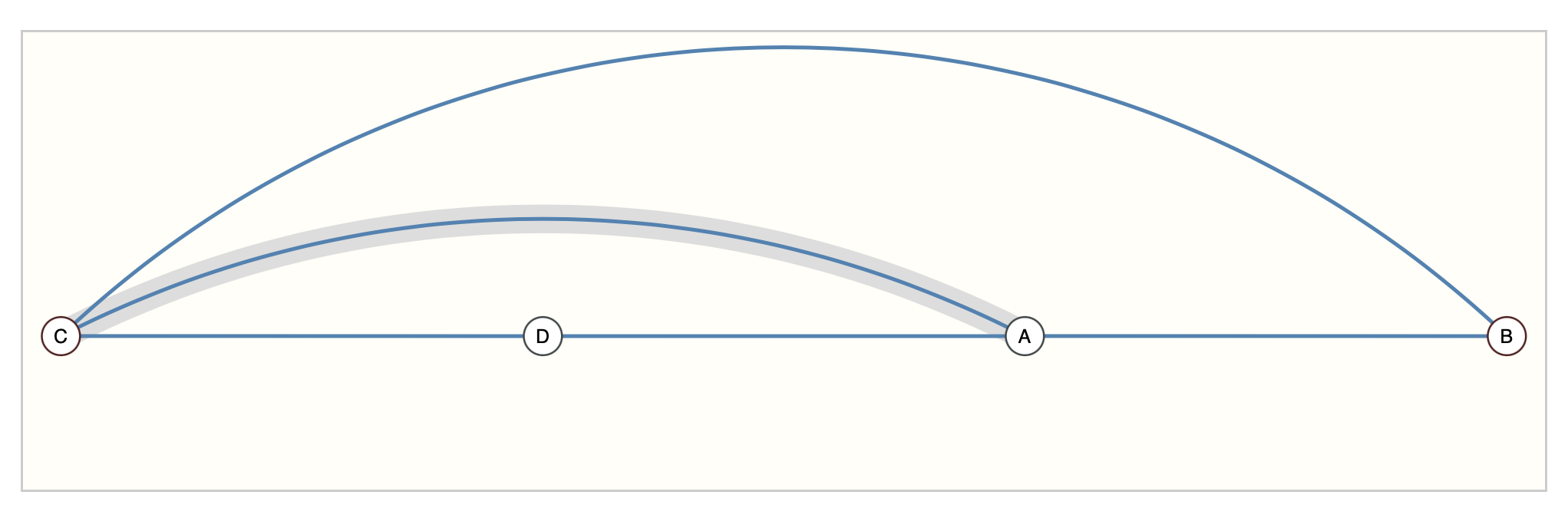
The example below shows every adjacency matrix that can describe this small graph of 4 nodes. This is already a significant number of adjacency matrices–for larger examples like Othello, the number is untenable.
下面的例子展示了每个可以描述这个4个节点的小图的邻接矩阵。这已经是相当多的邻接矩阵了——对于更大的例子，如Othello，这个数字是站不住脚的。

所有这些邻接矩阵都表示同一个图

One elegant and memory-efficient way of representing sparse matrices is as adjacency lists. These describe the connectivity of edge $e_k$ between nodes $n_i$ and $n_j$ as a tuple (i,j) in the k-th entry of an adjacency list. Since we expect the number of edges to be much lower than the number of entries for an adjacency matrix $(n_{nodes}^2)$, we avoid computation and storage on the disconnected parts of the graph.
使用邻接表是表示稀疏矩阵的一种简洁且内存效率较高的方法。它们将节点$n_i$和$n_j$之间的边$e_k$的连通性描述为邻接表第k个条目中的一个元组(i,j)。由于我们期望边的数量比邻接矩阵$(n_{nodes}^2)$的条目数量要少得多，所以我们避免了在图的非连通部分上的计算和存储。

Another way of stating this is with Big-O notation, it is preferable to have $O(n_{edges})$, rather than $O(n_{nodes}^2)$.
另一种表述方式是用大写O符号，最好是$O(n_{edges})$，而不是$O(n_{nodes}^2)$。

To make this notion concrete, we can see how information in different graphs might be represented under this specification:
为了使这个概念更具体，我们可以看到不同图表中的信息在这个规则下是如何表示的:

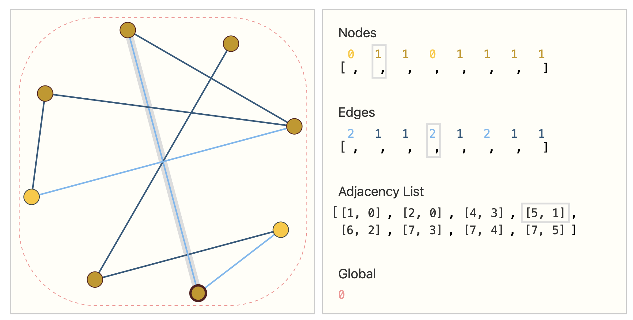
Hover and click on the edges, nodes, and global graph marker to view and change attribute representations. On one side we have a small graph and on the other the information of the graph in a tensor representation.
将鼠标悬停并单击边缘、节点和全局图形标记来查看和更改属性表示。一边是一个小图，另一边是张量表示的图的信息。

It should be noted that the figure uses scalar values per node/edge/global, but most practical tensor representations have vectors per graph attribute. Instead of a node tensor of size $[n_{nodes}]$ we will be dealing with node tensors of size $[n_{nodes},nod{e}_{dim}]$. Same for the other graph attributes.
值得注意的是，图在每个节点/边/全局中使用标量值，但是大多数实际的张量表示在每个图属性中都有向量。我们将处理大小为$[n_{nodes},nod{e}_{dim}]$的结点张量，而不是$[n_{nodes}]$的结点张量。其他图属性也是如此。

参考文献

[16] Learning Latent Permutations with Gumbel-Sinkhorn Networks Mena, G., Belanger, D., Linderman, S. and Snoek, J., 2018.

[17] Janossy Pooling: Learning Deep Permutation-Invariant Functions for Variable-Size Inputs Murphy, R.L., Srinivasan, B., Rao, V. and Ribeiro, B., 2018.