【论文阅读】A Gentle Introduction to Graph Neural Networks [图神经网络入门](6)
GNN playground
GNN游乐场
We’ve described a wide range of GNN components here, but how do they actually differ in practice? This GNN playground allows you to see how these different components and architectures contribute to a GNN’s ability to learn a real task.
我们已经了解了各种各样的GNN组件,但是它们在实践中有什么不同呢?这个GNN游乐场允许您了解这些不同的组件和体系结构如何帮助GNN学习实际任务的能力。
Our playground shows a graph-level prediction task with small molecular graphs. We use the the Leffingwell Odor Dataset [23] [24], which is composed of molecules with associated odor percepts (labels). Predicting the relation of a molecular structure (graph) to its smell is a 100 year-old problem straddling chemistry, physics, neuroscience, and machine learning.
我们的游乐场展示了一个带有小分子图的图预测任务。我们使用Leffingwell气味数据集[23] [24],它由分子和相关的气味感知器(标签)组成。预测分子结构(图)与气味的关系是一个百年难题,横跨化学、物理、神经科学和机器学习。
To simplify the problem, we consider only a single binary label per molecule, classifying if a molecular graph smells “pungent” or not, as labeled by a professional perfumer. We say a molecule has a “pungent” scent if it has a strong, striking smell. For example, garlic and mustard, which might contain the molecule allyl alcohol have this quality. The molecule piperitone, often used for peppermint-flavored candy, is also described as having a pungent smell.
为了简化这个问题,我们只考虑每个分子一个单一的二元标签,如果分子图闻起来“刺鼻”或不刺鼻,就按照专业调香师的标签进行分类。我们说一个分子有“刺鼻”气味,如果它有一种强烈的、刺鼻的气味。例如,大蒜和芥末中可能含有烯丙醇分子,具有这种特性。胡椒酮分子,通常用于薄荷味的糖果,也被描述为具有刺激性的气味。
We represent each molecule as a graph, where atoms are nodes containing a one-hot encoding for its atomic identity (Carbon, Nitrogen, Oxygen, Fluorine) and bonds are edges containing a one-hot encoding its bond type (single, double, triple or aromatic).
我们将每个分子表示为一个图,其中原子是包含一个one-hot编码(碳、氮、氧、氟)的节点,而键是包含一个one-hot编码(单键、双键、三键或芳香键)的键类型的边。
Our general modeling template for this problem will be built up using sequential GNN layers, followed by a linear model with a sigmoid activation for classification. The design space for our GNN has many levers that can customize the model:
1.The number of GNN layers, also called the depth.
2.The dimensionality of each attribute when updated. The update function is a 1-layer MLP with a relu activation function and a layer norm for normalization of activations.
3.The aggregation function used in pooling: max, mean or sum.
4.The graph attributes that get updated, or styles of message passing: nodes, edges and global representation. We control these via boolean toggles (on or off). A baseline model would be a graph-independent GNN (all message-passing off) which aggregates all data at the end into a single global attribute. Toggling on all message-passing functions yields a GraphNets architecture.
我们将使用顺序的GNN层来对这个问题进行建模,然后使用一个用于分类的sigmoid激活的线性模型。我们的GNN设计架构需要许多建模的手段:
1.GNN层数,又称深度。
2.更新时每个属性的维度。更新函数是一个具有relu激活函数和激活规范化层规范的单层MLP。
3.在池化操作中使用的聚合函数:max, mean或者sum。
4.被更新的图属性或消息传递的属性:节点、边和全局表示。我们通过布尔开关(on或off)来控制这些。基线模型将是一个独立于图的GNN(所有信息传递),它在最后将所有数据聚合到一个全局属性中。切换所有信息传递函数会生成一个GraphNets体系结构。
To better understand how a GNN is learning a task-optimized representation of a graph, we also look at the penultimate layer activations of the GNN. These ‘graph embeddings’ are the outputs of the GNN model right before prediction. Since we are using a generalized linear model for prediction, a linear mapping is enough to allow us to see how we are learning representations around the decision boundary.
为了更好地理解GNN如何学习图的任务最佳化表示,我们还将研究GNN的倒数第二层激活。这些“graph embeddings”是GNN模型在预测之前的输出。由于我们使用广义线性模型进行预测,一个线性映射就足以让我们看到如何围绕决策边界进行学习表示。
Since these are high dimensional vectors, we reduce them to 2D via principal component analysis (PCA). A perfect model would visibility separate labeled data, but since we are reducing dimensionality and also have imperfect models, this boundary might be harder to see.
由于这些是高维向量,我们通过主成分分析(PCA)将它们简化为2D。一个完美的模型可以看到单独的标签数据,但是由于我们在降低维数,所以美中不足的是,这个边界可能较难看到。
Play around with different model architectures to build your intuition. For example, see if you can edit the molecule on the left to make the model prediction increase. Do the same edits have the same effects for different model architectures?
使用不同的模型架构来构建您的认识。例如,看看你是否可以编辑左边的分子,使模型预测增加。对于不同的模型体系结构,相同的编辑是否具有相同的效果?
This playground is running live on the browser in tfjs.
这个游乐场可以在浏览器上实时运行tfjs框架。
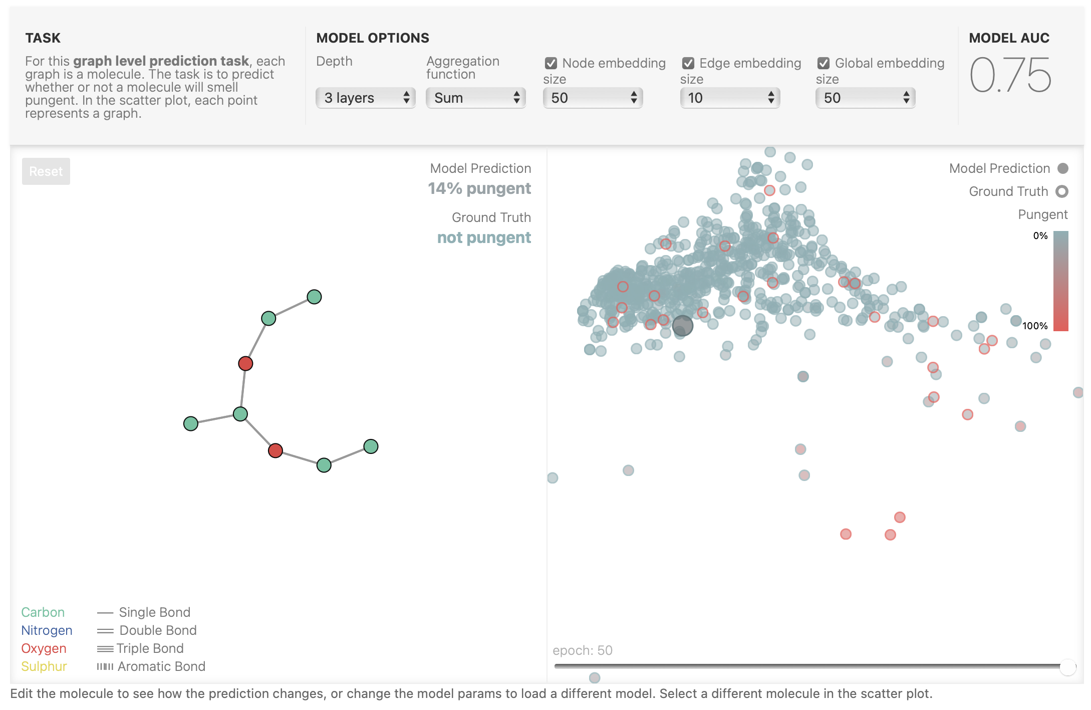
图1 Edit the molecule to see how the prediction changes, or change the model params to load a different model. Select a different molecule in the scatter plot.
编辑分子,看看预测如何变化,或改变模型参数,以加载不同的模型。在散点图中选择一个不同的分子。
该实验一共有6个参数可以变换,分别是Depth(模型层数/GNN层数)、Aggregation function(聚合函数)、Node embedding size(节点embedding大小)、Edge embedding size(边embedding大小)、Global embedding size(全局embedding大小)。
Aggregation function(聚合函数)类似于卷积神经网络池化层中的聚合函数,只不过卷积神经网络池化层中的聚合函数Sum函数并不常见。
Node embedding size也可以理解为表示节点的向量长度,Edge embedding size和Global embedding size亦然,这三个变量可以设置为空,也就是在条件未知的情况下去预测。
右边的散点图为数据集中每个分子图的预测结果与真实标签的重合程度。其中空心圈为Ground Truth,也就是一个点的圈边缘部分表示这个分子图的标签值; 实心圈为Model Prediction,也就是一个点的实心部分表示这个分子图的预测结果; 红色代表具有刺激性气味,蓝色代表不具有刺激性气味; 那么也就是说,如果一个点的圈边部分和实心部分如果颜色都是一样的,说明我们的模型对数据集中的该分子图的是否具有刺激性气味预测正确,反之,则预测失败; MODEL AUC为模型的预测准确率; Pungent为刺激性气味的程度。
下面为数据集中某个分子图的预测成功和预测失败的例子,可以看到预测成功的分子(图2)的Model Prediction为4% pungent,Ground Truth为not pungent,这说明预测该分子的刺激程度为4%,这与其标签为非刺激性基本吻合,说明预测成功; 预测失败的分子(图3)的Model Prediction为64% pungent,Ground Truth为not pungent,这说明预测该分子的刺激程度为64%,属于具有刺激性气味,这与其标签为非刺激性不吻合,说明预测失败; 该模型是在3层GNN,聚合函数为Sum,节点embedding大小为50,边embedding大小为10,全局embedding大小为50的参数下完成预测,其预测精确度为0.75。
 图2 预测成功的分子图
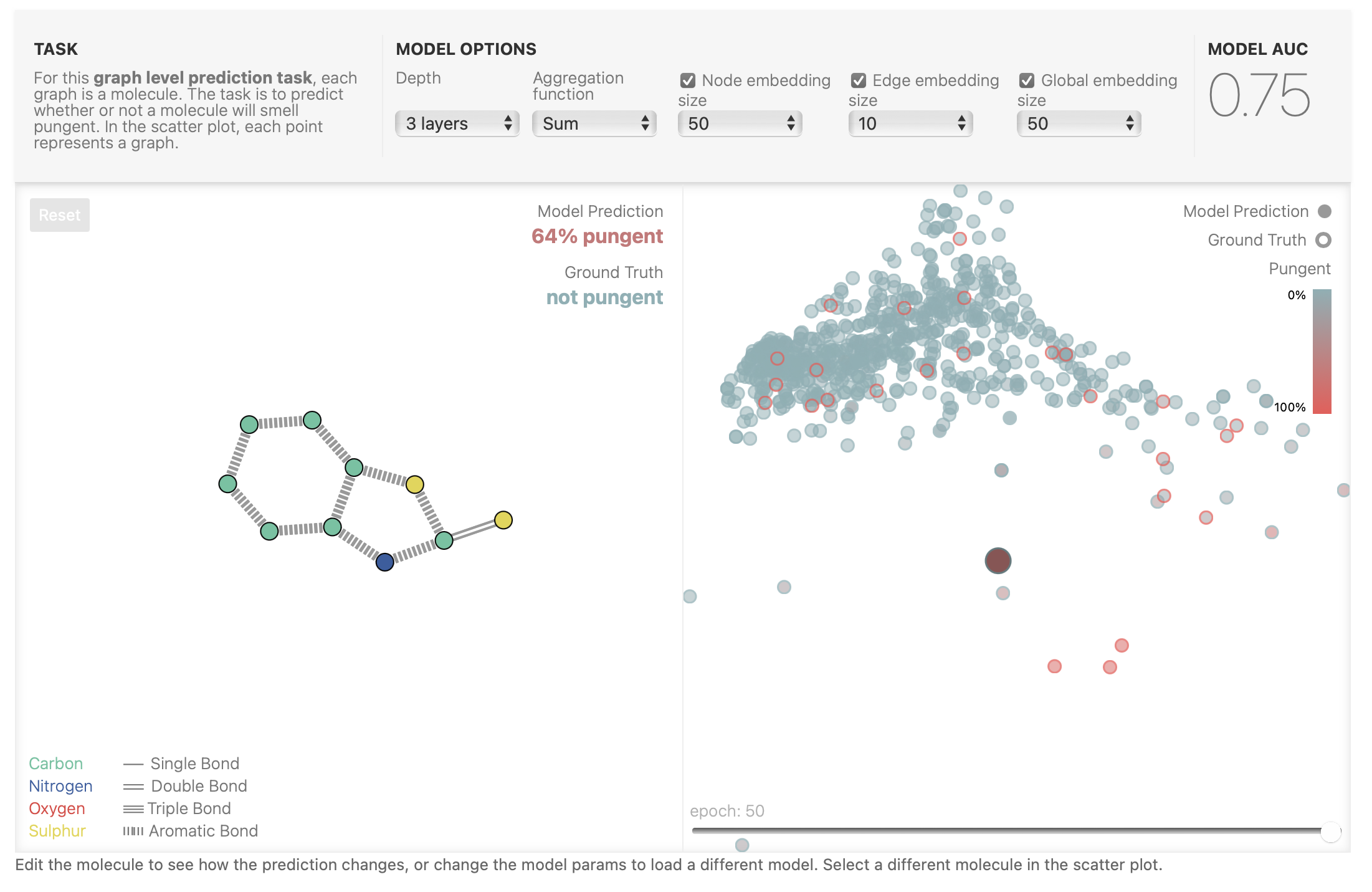 图3 预测失败的分子图
当然,你还可以在左边自定义分子图结构送入模型来预测该分子是否具有刺激性气味,图4为我们输入了一个分子图,其预测结果为9%刺激性气味,属于不具有刺激性气味,由于该图是我们自定义的,所以其标签为unknown。
 图4 自定义分子图及其预测结果
Some empirical GNN design lessons
一些GNN设计建议
When exploring the architecture choices above, you might have found some models have better performance than others. Are there some clear GNN design choices that will give us better performance? For example, do deeper GNN models perform better than shallower ones? or is there a clear choice between aggregation functions? The answers are going to depend on the data, [25] [26] , and even different ways of featurizing and constructing graphs can give different answers.
在探索上面的架构选择时,您可能会发现某些模型的准确率比其他模型更高。是否有一些明确的GNN设计架构,将给我们更好的性能?例如,较深的GNN模型是否比较浅的模型表现更好?或者在几种聚合函数之间有一个最好的选择?答案取决于数据,[25] [26],甚至不同的表示和构造图的方法也会得出不同的结论。
With the following interactive figure, we explore the space of GNN architectures and the performance of this task across a few major design choices: Style of message passing, the dimensionality of embeddings, number of layers, and aggregation operation type.
在下图中,我们通过几个主要的设计选择来探索GNN架构的空间和该任务的性能:信息传递的方式、embedding的维度、GNN的层数和聚合操作的类型。
Each point in the scatter plot represents a model: the x axis is the number of trainable variables, and the y axis is the performance. Hover over a point to see the GNN architecture parameters.
散点图中的每个点代表一个模型:x轴是可训练变量的数量,y轴是准确率。将鼠标悬停在一个点上可以看到GNN架构参数。
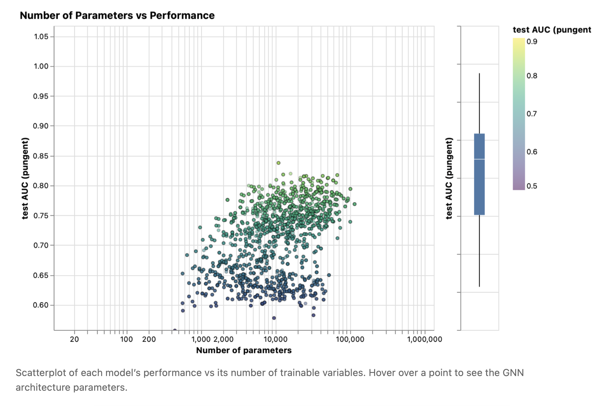 图5 每个模型的性能与它的可训练变量的数量的散点图。将鼠标悬停在一个点上可以看到GNN架构参数。
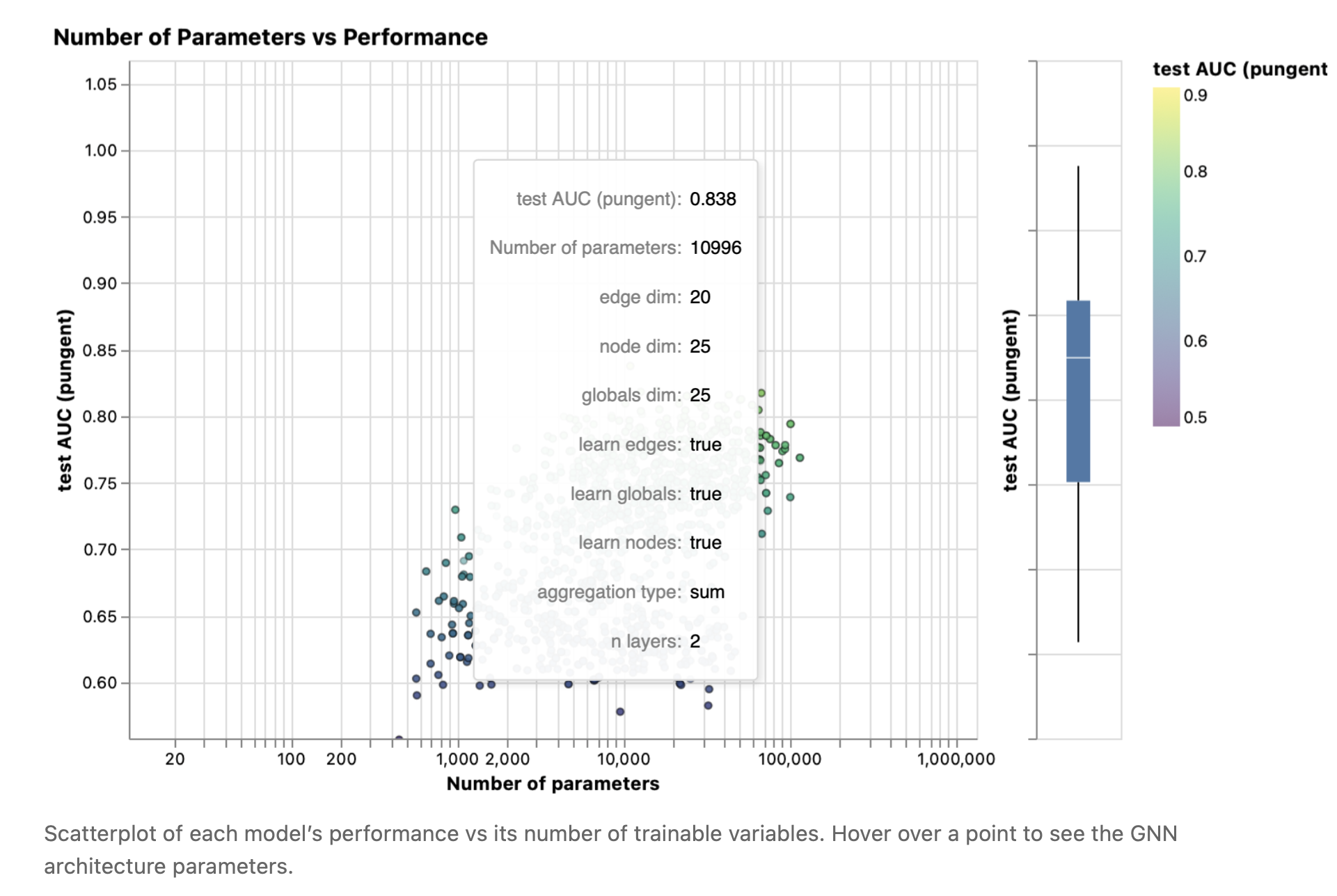 图6 最高准确率模型的参数
The first thing to notice is that, surprisingly, a higher number of parameters does correlate with higher performance. GNNs are a very parameter-efficient model type: for even a small number of parameters (3k) we can already find models with high performance.
首先要注意是,参数数量越多,性能出乎意料的越好。GNN是一种非常高效的参数模型: 即使是少量的参数(3k),我们仍然能够找到高性能的模型。
Next, we can look at the distributions of performance aggregated based on the dimensionality of the learned representations for different graph attributes.
接下来,我们可以查看基于不同图属性的表示学习的维数聚合的性能分布。
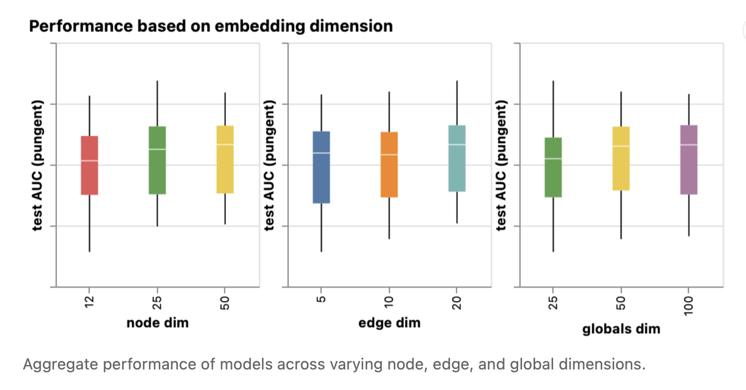 图7 在不同的节点、边和全局维度上聚合模型的性能。
We can notice that models with higher dimensionality tend to have better mean and lower bound performance but the same trend is not found for the maximum. Some of the top-performing models can be found for smaller dimensions. Since higher dimensionality is going to also involve a higher number of parameters, these observations go in hand with the previous figure.
我们可以注意到,模型的维数越高,其均值和最小值(准确率最低的模型)的性能越好,但最大值没有出现相同的趋势。对于较低维度的模型,可以找到一些性能最好的模型。由于更高的维数也将涉及更多的参数,这些观察结果与前面的图是一致的。
其实这段话也就是想告诉我们,节点、边、全局向量的维度并不是越多模型的性能就越强,模型的性能与许多参数息息相关。
Next we can see the breakdown of performance based on the number of GNN layers.
接下来,我们可以看到GNN层数对模型性能的影响。
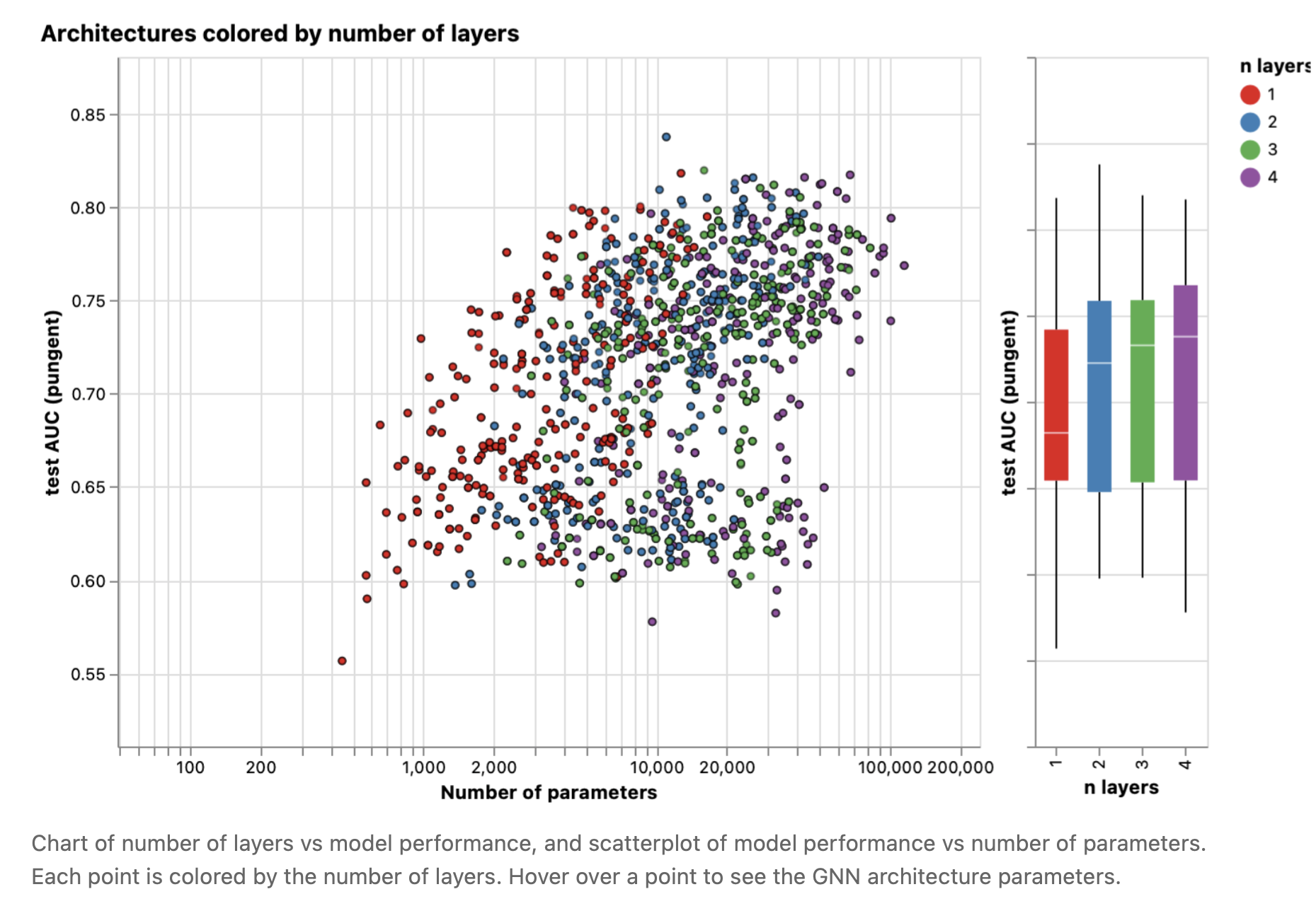
图8 GNN层数与模型性能的关系图,模型性能与参数数量的关系散点图。每个点都根据层数着色。将鼠标悬停在一个点上可以看到GNN架构参数。
The box plot shows a similar trend, while the mean performance tends to increase with the number of layers, the best performing models do not have three or four layers, but two. Furthermore, the lower bound for performance decreases with four layers. This effect has been observed before, GNN with a higher number of layers will broadcast information at a higher distance and can risk having their node representations ‘diluted’ from many successive iterations [27].
箱形图也显示了类似的趋势,虽然平均性能随着层数的增加而增加,但性能最好的模型不是三层或四层,而是两层。此外,性能的最小值随着层的增加而降低。这种效应之前已经观察到,具有较多层数的GNN将以更远的距离传递信息,并可能在许多连续迭代中使其节点表示被“稀释”[27]。
Does our dataset have a preferred aggregation operation? Our following figure breaks down performance in terms of aggregation type.
我们的数据集有聚合操作的最佳选择吗?下图按照聚合操作的类型对模型性能进行了解析。

图9 聚合类型与模型性能的关系图,模型性能与参数个数的关系散点图。每个点都根据聚合类型着色。将鼠标悬停在一个点上可以看到GNN架构参数。
Overall it appears that sum has a very slight improvement on the mean performance, but max or mean can give equally good models. This is useful to contextualize when looking at the discriminatory/expressive capabilities of aggregation operations .
总的来说,sum函数似乎对平均性能有非常轻微的改善,但max或mean可以给出性能同样好的模型。选择聚合操作的类型/表达能力时对于将其置于全局上下文中非常有用。
The previous explorations have given mixed messages. We can find mean trends where more complexity gives better performance but we can find clear counterexamples where models with fewer parameters, number of layers, or dimensionality perform better. One trend that is much clearer is about the number of attributes that are passing information to each other.
之前的探索给出了复杂的信息。我们可以发现模型复杂程度越高,性能越好的平均趋势,但我们也可以发现参数越少、层数越少或维数越少的明显反例。一个更明显的趋势是相互传递信息的属性的数量。
Here we break down performance based on the style of message passing. On both extremes, we consider models that do not communicate between graph entities (“none”) and models that have messaging passed between nodes, edges, and globals.
这里,我们将根据信息传递的方式对模型性能进行解析。在这两种极端情况下,我们考虑的模型在图实体(“none”)之间不进行信息传递,而模型在节点、边和全局之间进行信息传递。
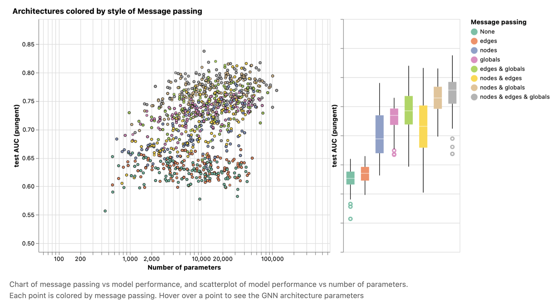
图10 信息传递与模型性能的关系图,模型性能与参数数量的关系散点图。每个点都通过信息传递着色。将鼠标悬停在一个点上可以看到GNN架构参数
Overall we see that the more graph attributes are communicating, the better the performance of the average model. Our task is centered on global representations, so explicitly learning this attribute also tends to improve performance. Our node representations also seem to be more useful than edge representations, which makes sense since more information is loaded in these attributes.
总的来说,我们看到能够进行信息传递的图属性越多,平均模型的性能就越好。我们的任务以全局表示为中心,因此明确地学习这个属性也有助于提高性能。我们的节点表示似乎也比边表示更有用,这是有意义的,因为在这些属性中加载了更多的信息。
There are many directions you could go from here to get better performance. We wish two highlight two general directions, one related to more sophisticated graph algorithms and another towards the graph itself.
为了获得更好的性能,你可以从很多方面着手。我们希望突出两个方向,一个与更复杂的图算法有关,另一个与图本身有关。
Up until now, our GNN is based on a neighborhood-based pooling operation. There are some graph concepts that are harder to express in this way, for example a linear graph path (a connected chain of nodes). Designing new mechanisms in which graph information can be extracted, executed and propagated in a GNN is one current research area [28] , [29] , [30] , [31] .
到目前为止,我们的GNN是基于邻居共享操作的。有些图概念很难用这种方式表达,例如线性图路径(连接的节点链)。设计一种新的机制,使图信息能够在GNN中提取、执行和传递是当前的研究领域之一[28] , [29] , [30] , [31]。
One of the frontiers of GNN research is not making new models and architectures, but “how to construct graphs”, to be more precise, imbuing graphs with additional structure or relations that can be leveraged. As we loosely saw, the more graph attributes are communicating the more we tend to have better models. In this particular case, we could consider making molecular graphs more feature rich, by adding additional spatial relationships between nodes, adding edges that are not bonds, or explicit learnable relationships between subgraphs.
GNN研究的前沿领域之一不是制造新的模型和架构,而是“如何构造图”,更精确地说,为图注入可以利用的额外结构或关系。正如我们所看到的,图属性之间的信息传递越多,我们的模型性能就越好。在这种特殊情况下,我们可以考虑通过添加节点之间的额外空间关系、添加非键的边或子图之间的显式可学习关系,使子图的特征更加丰富。
See more in Other types of graphs.
更多信息见其他类型的图。
参考文献
[23] Leffingwell Odor Dataset Sanchez-Lengeling, B., Wei, J.N., Lee, B.K., Gerkin, R.C., Aspuru-Guzik, A. and Wiltschko, A.B., 2020.
[24] Machine Learning for Scent: Learning Generalizable Perceptual Representations of Small Molecules Sanchez-Lengeling, B., Wei, J.N., Lee, B.K., Gerkin, R.C., Aspuru-Guzik, A. and Wiltschko, A.B., 2019.
[25] Benchmarking Graph Neural Networks Dwivedi, V.P., Joshi, C.K., Laurent, T., Bengio, Y. and Bresson, X., 2020.
[26] Design Space for Graph Neural Networks You, J., Ying, R. and Leskovec, J., 2020.
[27] Principal Neighbourhood Aggregation for Graph Nets Corso, G., Cavalleri, L., Beaini, D., Lio, P. and Velickovic, P., 2020.
[28] Graph Traversal with Tensor Functionals: A Meta-Algorithm for Scalable Learning Markowitz, E., Balasubramanian, K., Mirtaheri, M., Abu-El-Haija, S., Perozzi, B., Ver Steeg, G. and Galstyan, A., 2021.
[29] Graph Neural Tangent Kernel: Fusing Graph Neural Networks with Graph Kernels Du, S.S., Hou, K., Poczos, B., Salakhutdinov, R., Wang, R. and Xu, K., 2019.
[30] Representation Learning on Graphs with Jumping Knowledge Networks Xu, K., Li, C., Tian, Y., Sonobe, T., Kawarabayashi, K. and Jegelka, S., 2018.
[31] Neural Execution of Graph Algorithms Velickovic, P., Ying, R., Padovano, M., Hadsell, R. and Blundell, C., 2019.