【论文阅读】A Gentle Introduction to Graph Neural Networks [图神经网络入门]（5）

Graph Neural Networks
图神经网络

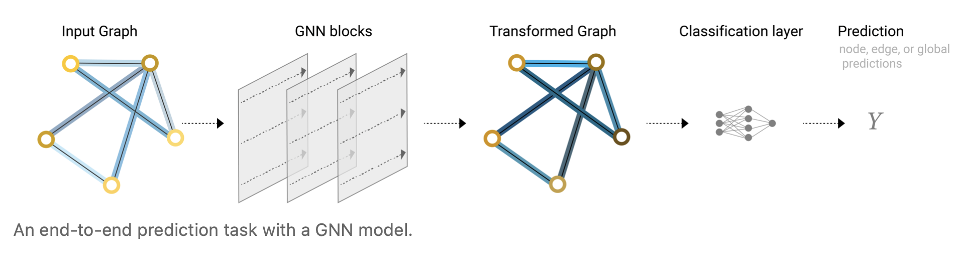
Now that the graph’s description is in a matrix format that is permutation invariant, we will describe using graph neural networks (GNNs) to solve graph prediction tasks. A GNN is an optimizable transformation on all attributes of the graph (nodes, edges, global-context) that preserves graph symmetries (permutation invariances). We’re going to build GNNs using the “message passing neural network” framework proposed by Gilmer et al. [18] using the Graph Nets architecture schematics introduced by Battaglia et al. [19] GNNs adopt a “graph-in, graph-out” architecture meaning that these model types accept a graph as input, with information loaded into its nodes, edges and global-context, and progressively transform these embeddings, without changing the connectivity of the input graph.
既然图的描述是排列不变的矩阵格式，我们将使用图神经网络(GNN)来描述以解决图预测任务。GNN是对图的所有属性(节点、边、全局上下文)的一种可优化的转换，它保持了图的对称性(排列不变性)。我们将使用Gilmer等人提出的“信息传递神经网络”[18]框架来构建GNN。使用Battaglia等人介绍的图网架构示意图[19]。GNN采用一种“图入，图出”的体系结构，这意味着这些模型类型接受一个图作为输入，将信息加载到它的节点、边和全局上下文中，并逐步转换这些embedding，而不改变输入图的连通性。

The simplest GNN
最简单的GNN

With the numerical representation of graphs that we’ve constructed above (with vectors instead of scalars), we are now ready to build a GNN. We will start with the simplest GNN architecture, one where we learn new embeddings for all graph attributes (nodes, edges, global), but where we do not yet use the connectivity of the graph.
使用我们上面构建的图的数字表示(使用向量而不是标量)，我们现在可以构建GNN了。我们将从最简单的GNN架构开始，在这个架构中，我们学习所有图属性(节点、边、全局)的新embeddings，但我们还没有使用图的连通性。

For simplicity, the previous diagrams used scalars to represent graph attributes; in practice feature vectors, or embeddings, are much more useful.
You could also call it a GNN block. Because it contains multiple operations/layers (like a ResNet block).
为简单起见，前面的图使用标量来表示图的属性;在实践中，特征向量或embeddings更有用。
你也可以叫它GNN block。因为它包含多个操作/层(与ResNet block类似)。

This GNN uses a separate multilayer perceptron (MLP) (or your favorite differentiable model) on each component of a graph; we call this a GNN layer. For each node vector, we apply the MLP and get back a learned node-vector. We do the same for each edge, learning a per-edge embedding, and also for the global-context vector, learning a single embedding for the entire graph.
该GNN使用一个独立的多层感知器(MLP)(或你喜欢的可微模型)在图的每个组件; 我们称之为GNN层。对于每个节点向量，我们应用MLP并得到一个学习后的节点向量。我们对每条边做同样的操作，学习每条边的embedding，对全局上下文向量也做同样的操作，学习整个图的单个embedding。

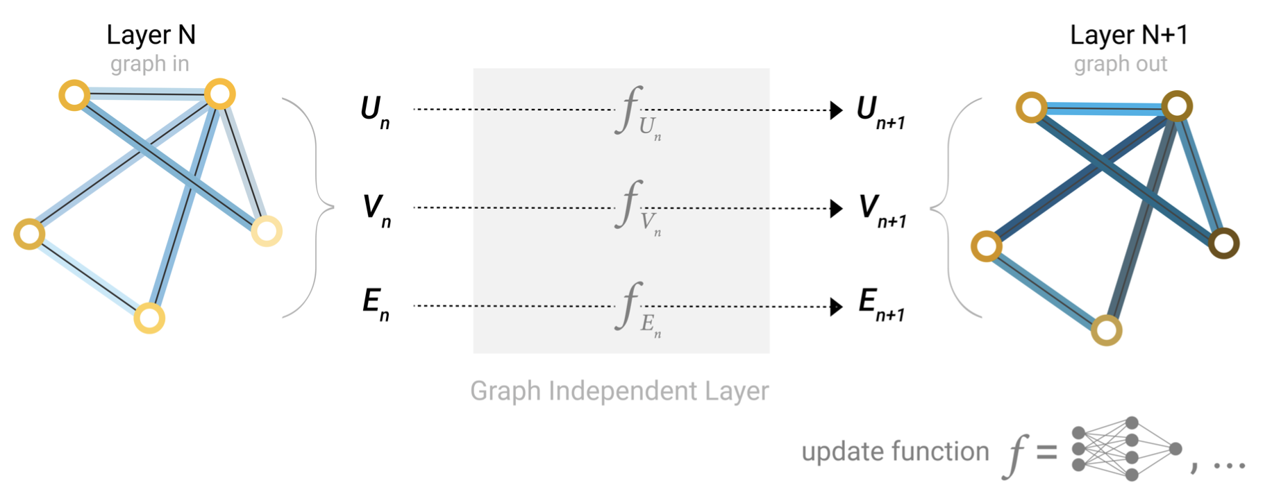
A single layer of a simple GNN. A graph is the input, and each component (V,E,U) gets updated by a MLP to produce a new graph. Each function subscript indicates a separate function for a different graph attribute at the n-th layer of a GNN model.
一个简单的GNN单层。输入是一个图，MLP更新每个参数(V,E,U)以生成一个新的图。每个函数下标表示GNN模型第n层的不同图形属性的单独函数。

As is common with neural networks modules or layers, we can stack these GNN layers together.
与神经网络模块或层一样，我们可以将这些GNN层堆叠在一起。

Because a GNN does not update the connectivity of the input graph, we can describe the output graph of a GNN with the same adjacency list and the same number of feature vectors as the input graph. But, the output graph has updated embeddings, since the GNN has updated each of the node, edge and global-context representations.
由于GNN不更新输入的图的连通性，我们可以用与输入的图相同的邻接表和相同数量的特征向量来描述GNN的输出图。但是，输出图更新了embeddings，因为GNN更新了每个节点、边和全局上下文表示。

GNN Predictions by Pooling Information
通过池化信息来预测GNN

We have built a simple GNN, but how do we make predictions in any of the tasks we described above?
我们已经构建了一个简单的GNN，但是我们如何在上面描述的任务中进行预测呢?

We will consider the case of binary classification, but this framework can easily be extended to the multi-class or regression case. If the task is to make binary predictions on nodes, and the graph already contains node information, the approach is straightforward — for each node embedding, apply a linear classifier.
我们先来考虑二分类问题，这个框架可以很容易地扩展到多分类或回归的问题。如果任务是对节点进行二分类预测，而图中已经包含了节点信息，那么这种方法很简单——对于每个embedding的节点，应用一个线性分类器。

We could imagine a social network, where we wish to anonymize user data (nodes) by not using them, and only using relational data (edges). One instance of such a scenario is the node task we specified in the Node-level task subsection. In the Karate club example, this would be just using the number of meetings between people to determine the alliance to Mr. Hi or John H.
我们可以想象一个社交网络，在这个网络中，我们希望匿名化用户数据(节点)，不使用它们，只使用关系数据(边)。这种场景的一个实例是我们在节点层面的任务小节中指定的节点任务。在空手道俱乐部的例子中，这将只是使用人们之间的会议数量来决定与Mr. Hi或John H的联盟。

However, it is not always so simple. For instance, you might have information in the graph stored in edges, but no information in nodes, but still need to make predictions on nodes. We need a way to collect information from edges and give them to nodes for prediction. We can do this by pooling. Pooling proceeds in two steps:

1.For each item to be pooled, gather each of their embeddings and concatenate them into a matrix.

2.The gathered embeddings are then aggregated, usually via a sum operation.

然而，事情并不总是那么简单。例如，你可能在图里存储在边中的信息，但在节点中没有信息，但仍然需要对节点进行预测。我们需要一种方法从边收集信息，并将它们交给节点进行预测。我们可以通过pooling（池化）来实现。池化操作实现分两个步骤:

1.对于要进行池化操作的每个项，将它们的每个embeddings集合起来，并将它们连接到一个矩阵中。

2.然后，通常使用求和操作对收集到的embeddings进行聚合。

For a more in-depth discussion on aggregation operations go to the Comparing aggregation operations section.
有关聚合操作的更深入讨论，请参考聚合操作比较一节。

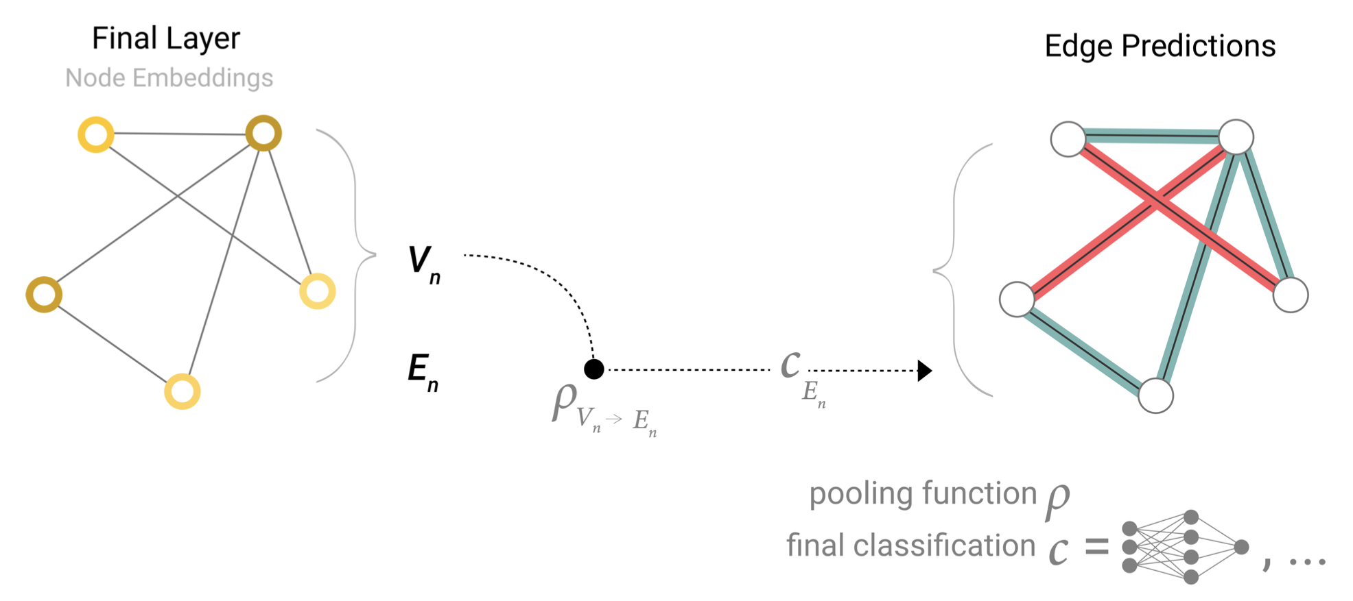
We represent the pooling operation by the letter $\rho$, and denote that we are gathering information from edges to nodes as ${\rho }_{E_n\to V_n}$.
我们用字母$\rho$表示池化操作，并表示我们从边收集信息到节点${\rho }_{E_n\to V_n}$。

从相邻边聚合信息

Hover over a node (black node) to visualize which edges are gathered and aggregated to produce an embedding for that target node.
将鼠标悬停在一个节点(黑节点)上，可以查看收集和聚合了哪些边以生成目标节点的嵌入。

So If we only have edge-level features, and are trying to predict binary node information, we can use pooling to route (or pass) information to where it needs to go. The model looks like this.
因此，如果我们只有边层面的特征，并试图预测二分类节点信息，我们可以使用池化操作路由(或传递)信息到它需要去的地方。模型是这样的。

If we only have node-level features, and are trying to predict binary edge-level information, the model looks like this.
如果我们只有节点层面的特征，并试图预测二分类问题边层面的信息，那么模型看起来是这样的。

One example of such a scenario is the edge task we specified in Edge level task sub section. Nodes can be recognized as image entities, and we are trying to predict if the entities share a relationship (binary edges).
这种场景的一个例子是我们在边层面任务子节中指定的边层面任务。节点可以被识别为图像中的实体，我们试图预测这些实体是否共享一个关系(边的二分类)。

If we only have node-level features, and need to predict a binary global property, we need to gather all available node information together and aggregate them. This is similar to Global Average Pooling layers in CNNs. The same can be done for edges.
如果我们只有节点层面的特征，并且需要预测二分类问题的全局属性，那么我们需要将所有可用的节点信息收集在一起，并对它们进行聚合。这类似于CNN中的全局平均池化层（Average Pooling）。对于边也可以这样做。

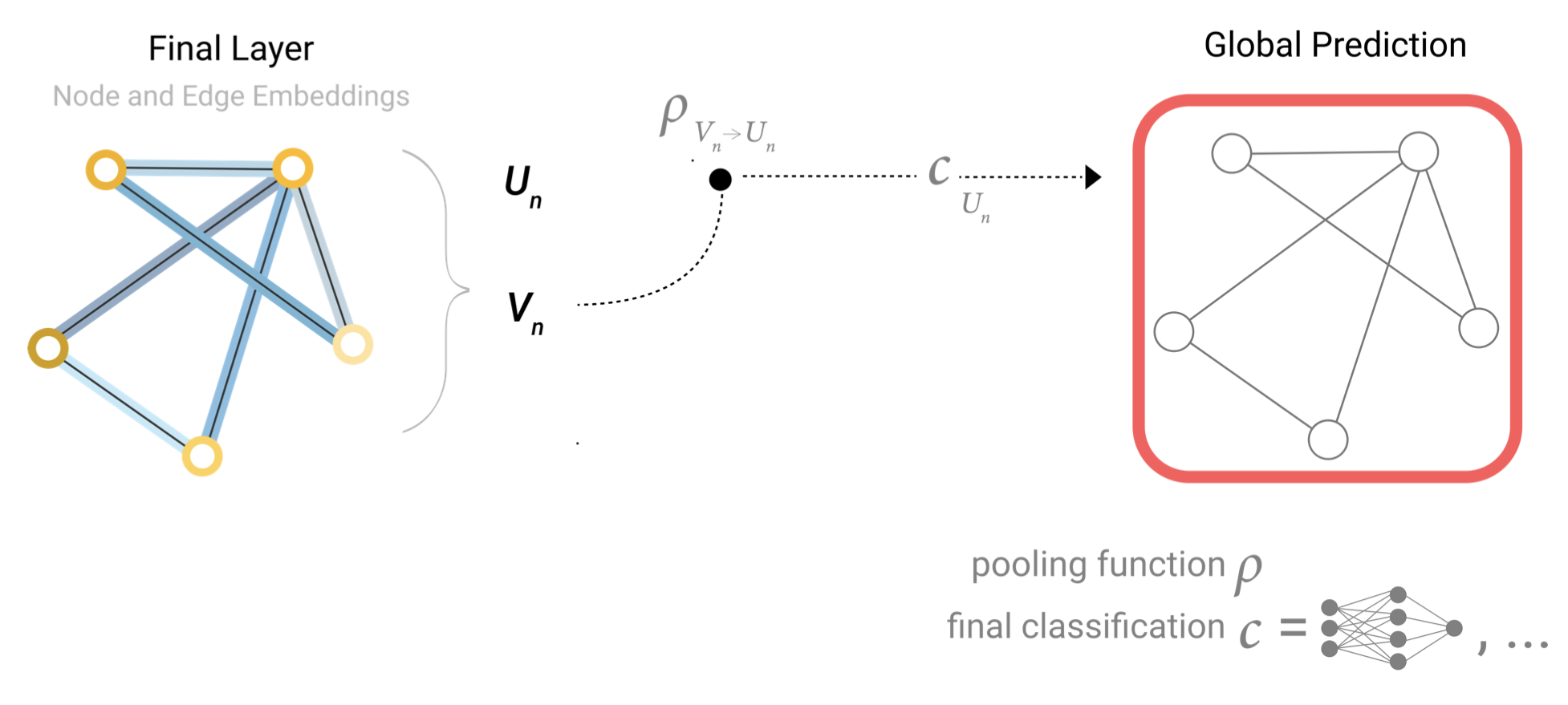
This is a common scenario for predicting molecular properties. For example, we have atomic information, connectivity and we would like to know the toxicity of a molecule (toxic/not toxic), or if it has a particular odor (rose/not rose).
这是预测分子性质的一个常见场景。例如，我们有原子信息，连通性，我们想知道一个分子的毒性(有毒/无毒)，或者它是否有特定的气味(玫瑰香/非玫瑰香)。

In our examples, the classification model $c$ can easily be replaced with any differentiable model, or adapted to multi-class classification using a generalized linear model.
在我们的例子中，分类模型$c$可以很容易地用任何可微分模型替换，或者使用广义线性模型适应多分类问题。

基于GNN模型的端到端预测任务

Now we’ve demonstrated that we can build a simple GNN model, and make binary predictions by routing information between different parts of the graph. This pooling technique will serve as a building block for constructing more sophisticated GNN models. If we have new graph attributes, we just have to define how to pass information from one attribute to another.
现在，我们已经演示了构建一个简单的GNN模型，并通过在图的不同部分之间传递信息来进行二分类预测。这种池化技术将作为构建更复杂的GNN模型的基础。如果我们有新的图属性，我们只需要定义如何将信息从一个属性传递到另一个属性即可。

Note that in this simplest GNN formulation, we’re not using the connectivity of the graph at all inside the GNN layer. Each node is processed independently, as is each edge, as well as the global context. We only use connectivity when pooling information for prediction.
请注意，在这个最简单的GNN架构中，我们根本没有在GNN层中使用图的连通性。每个节点、每条边以及全局上下文都是独立处理的。我们只在将信息用于预测时使用连通性。

Passing messages between parts of the graph
图各个部分之间的信息传递

We could make more sophisticated predictions by using pooling within the GNN layer, in order to make our learned embeddings aware of graph connectivity. We can do this using message passing[18], where neighboring nodes or edges exchange information and influence each other’s updated embeddings.
通过在GNN层中使用池化操作，我们可以做出更复杂的预测，使我们学到的embeddings关联到图的连通性。我们可以使用信息传递[18]来实现这一点，即相邻节点或边交换信息并影响彼此的更新embeddings。

Message passing works in three steps:

1.For each node in the graph, gather all the neighboring node embeddings (or messages), which is the $g$ function described above.

2.Aggregate all messages via an aggregate function (like sum).

3.All pooled messages are passed through an update function, usually a learned neural network.

信息传递工作分为三个步骤:

1.对于图中的每个节点，收集所有的相邻节点embeddings (或信息)，即上面描述的$g$函数。

2.通过聚合函数(与sum函数类似)聚合所有信息。

3.所有汇集的信息都通过一个更新函数传递，通常是一个学习过的神经网络。

You could also 1) gather messages, 3) update them and 2) aggregate them and still have a permutation invariant operation.[20]
您还可以1)收集信息，3)更新信息，2)聚合信息，并且仍然具有置换不变操作。[20]

Just as pooling can be applied to either nodes or edges, message passing can occur between either nodes or edges.
正如池化操作可以应用于节点或边一样，信息传递也可以发生在节点或边之间。

These steps are key for leveraging the connectivity of graphs. We will build more elaborate variants of message passing in GNN layers that yield GNN models of increasing expressiveness and power.
这些步骤是利用图连通性的关键。我们将在GNN层中构建信息传递的更复杂的变体，从而产生可提高表达能力和功能的GNN模型。

Hover over a node, to highlight adjacent nodes and visualize the adjacent embedding that would be pooled, updated and stored.
将鼠标悬停在一个节点上，以突出显示相邻的节点，并显示将要合并、更新和存储的相邻embedding。

This sequence of operations, when applied once, is the simplest type of message-passing GNN layer.
如果应用一次，这个操作序列就是信息传递GNN层的最简单类型。

This is reminiscent of standard convolution: in essence, message passing and convolution are operations to aggregate and process the information of an element’s neighbors in order to update the element’s value. In graphs, the element is a node, and in images, the element is a pixel. However, the number of neighboring nodes in a graph can be variable, unlike in an image where each pixel has a set number of neighboring elements.
这让我们想起了标准卷积神经网络:从本质上讲，信息传递和卷积是聚合和处理元素邻居信息以更新元素值的操作。在图形中，元素是一个节点，而在图像中，元素是一个像素。然而，图中相邻节点的数量可以是可变的，不像在图像中，每个像素都有一组相邻元素。

By stacking message passing GNN layers together, a node can eventually incorporate information from across the entire graph: after three layers, a node has information about the nodes three steps away from it.
通过将传递GNN层的信息叠加在一起，一个节点最终可以整合来自整个图的信息: 经过三层后，一个节点就拥有了距离它三步远的节点的信息。

We can update our architecture diagram to include this new source of information for nodes:
我们可以更新我们的架构图来包含这个新的节点信息源:

Schematic for a GCN architecture, which updates node representations of a graph by pooling neighboring nodes at a distance of one degree.
一种GCN架构的示意图，它通过将距离为一的相邻节点池化来更新图的节点表示。

Learning edge representations
学习边表示

Our dataset does not always contain all types of information (node, edge, and global context). When we want to make a prediction on nodes, but our dataset only has edge information, we showed above how to use pooling to route information from edges to nodes, but only at the final prediction step of the model. We can share information between nodes and edges within the GNN layer using message passing.
我们的数据集并不总是包含所有类型的信息(节点、边和全局上下文)。当我们想要对节点进行预测，但我们的数据集只有边的信息时，我们在上面展示了如何使用池化操作将信息从边传递到节点，但只在模型的最终预测步骤。我们可以使用消息传递在GNN层的节点和边之间共享信息。

We can incorporate the information from neighboring edges in the same way we used neighboring node information earlier, by first pooling the edge information, transforming it with an update function, and storing it.
我们可以将来自相邻边的信息合并到一起，就像我们之前使用相邻节点信息的方式一样，首先将边的信息合并到一起，用一个更新函数对其进行转换，然后存储它。

However, the node and edge information stored in a graph are not necessarily the same size or shape, so it is not immediately clear how to combine them. One way is to learn a linear mapping from the space of edges to the space of nodes, and vice versa. Alternatively, one may concatenate them together before the update function.
然而，存储在图中的节点和边的信息不一定是相同的大小或形状，因此，如何将它们组合起来还不是立即就清楚的。一种方法是学习从边空间到节点空间的线性映射，反之亦然。或者，可以在更新函数之前将它们连接在一起。

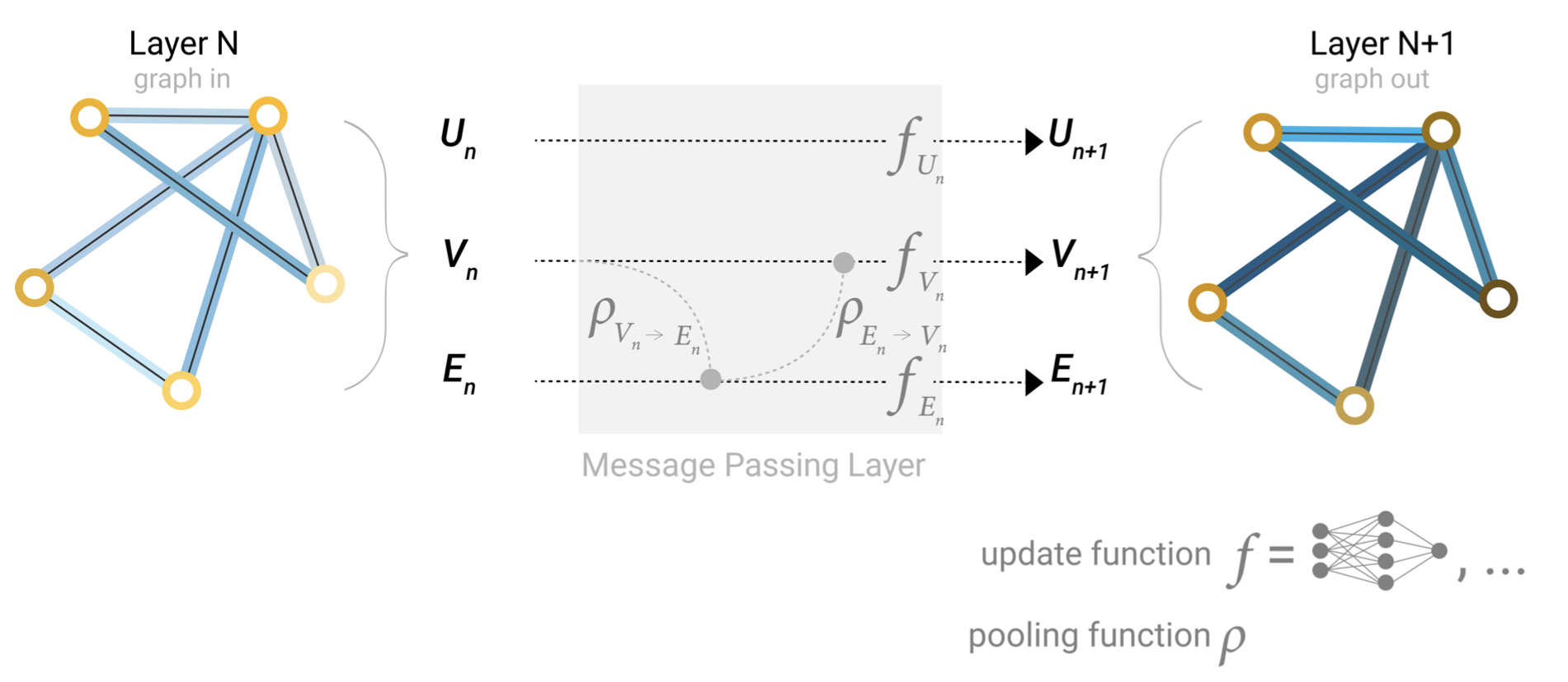
Architecture schematic for Message Passing layer. The first step “prepares” a message composed of information from an edge and it’s connected nodes and then “passes” the message to the node.
消息传递层的架构示意图。第一步“准备”一条由来自边及其连接节点的信息组成的消息，然后将消息“传递”给该节点。

Which graph attributes we update and in which order we update them is one design decision when constructing GNNs. We could choose whether to update node embeddings before edge embeddings, or the other way around. This is an open area of research with a variety of solutions– for example we could update in a ‘weave’ fashion [21] where we have four updated representations that get combined into new node and edge representations: node to node (linear), edge to edge (linear), node to edge (edge layer), edge to node (node layer).
在构造GNN时，我们需要决定更新哪些图属性以及更新它们的顺序。我们可以选择是否在边缘嵌入之前更新节点嵌入，或者反之。这是一个开放的研究领域与各种解决方案——例如我们可以更新“编织”的方式[21],我们有四个更新表示,组合成新节点和边缘表示:节点到节点(线性),边到边(线性),节点到边(边层面),边到节点(节点层面)。

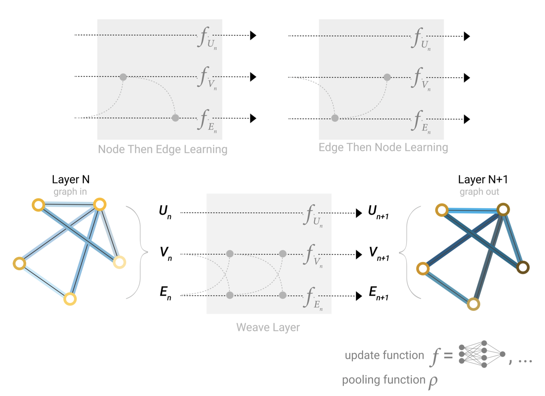
Some of the different ways we might combine edge and node representation in a GNN layer.
在GNN层中结合边和节点表示的一些不同方法。

Adding global representations
增加全局表示

There is one flaw with the networks we have described so far: nodes that are far away from each other in the graph may never be able to efficiently transfer information to one another, even if we apply message passing several times. For one node, If we have k-layers, information will propagate at most k-steps away. This can be a problem for situations where the prediction task depends on nodes, or groups of nodes, that are far apart. One solution would be to have all nodes be able to pass information to each other. Unfortunately for large graphs, this quickly becomes computationally expensive (although this approach, called ‘virtual edges’, has been used for small graphs such as molecules). [18]
到目前为止，我们所描述的网络还存在一个缺陷:图中彼此相距较远的节点可能永远无法有效地相互传递信息，即使我们应用了多次消息传递。对于一个节点，如果我们有k层，信息将在最多k步的距离传播。在预测任务依赖于距离很远的节点或节点组的情况下，这会成为一个问题。一种解决方案是让所有节点都能够互相传递信息。不幸的是，对于大的图来说，这很快就会增加计算成本(尽管这种被称为“虚边”的方法已经被用于小的图，如分子)。[18]

One solution to this problem is by using the global representation of a graph (U) which is sometimes called a master node[19] [18] or context vector. This global context vector is connected to all other nodes and edges in the network, and can act as a bridge between them to pass information, building up a representation for the graph as a whole. This creates a richer and more complex representation of the graph than could have otherwise been learned.
解决这个问题的一种方法是使用图(U)的全局表示，它有时被称为主节点[19] [18]或上下文向量。这个全局上下文向量连接到网络中所有其他的节点和边，作为它们之间传递信息的桥梁，建立了整个图的表示。这将创建一个更丰富、更复杂的图形表示，而不是通过其他方法来学习。

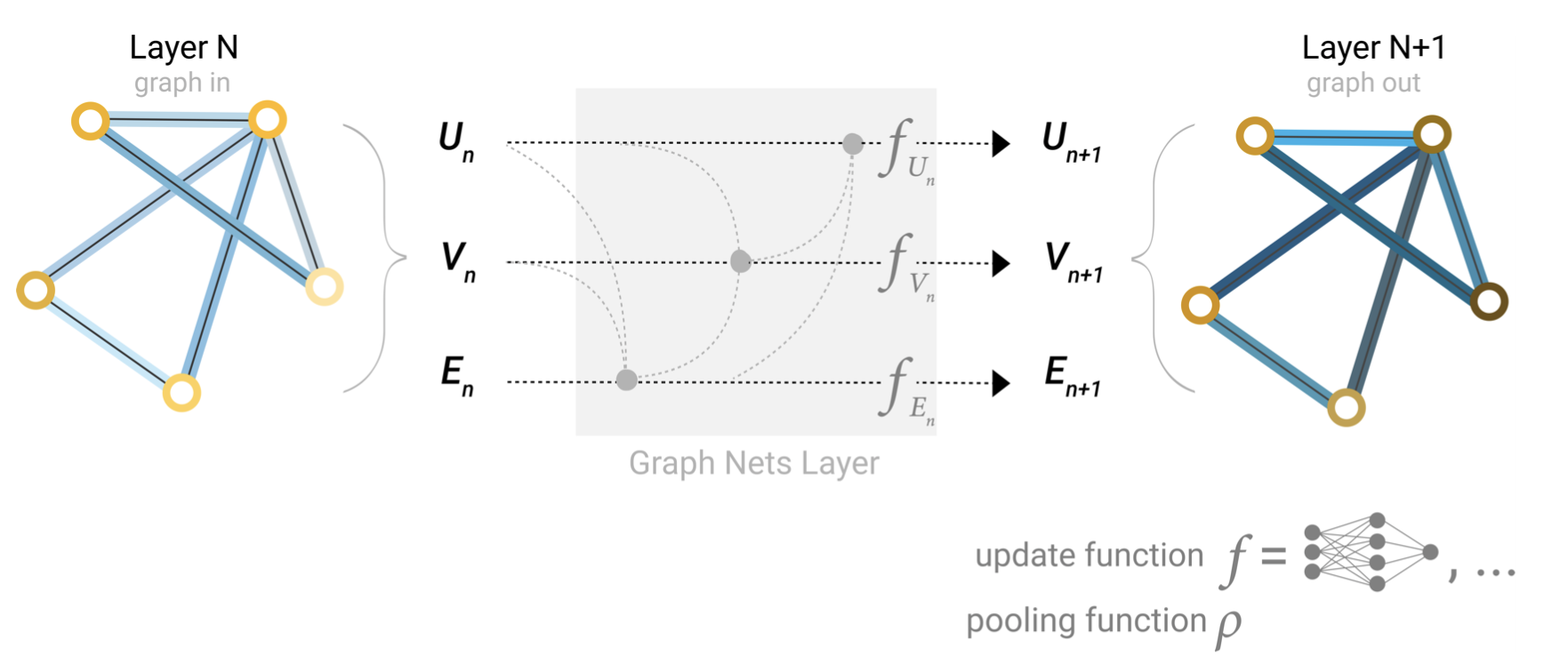
Schematic of a Graph Nets architecture leveraging global representations.
利用全局表示的Graph Nets体系结构示意图。

In this view all graph attributes have learned representations, so we can leverage them during pooling by conditioning the information of our attribute of interest with respect to the rest. For example, for one node we can consider information from neighboring nodes, connected edges and the global information. To condition the new node embedding on all these possible sources of information, we can simply concatenate them. Additionally we may also map them to the same space via a linear map and add them or apply a feature-wise modulation layer [22], which can be considered a type of featurize-wise attention mechanism.
在这个视图中，所有的图形属性都已经学习了表示，所以我们可以在池化过程中利用它们，方法是将我们感兴趣的属性的信息与其他属性相比较。例如，对于一个节点，我们可以考虑来自相邻节点、连通边和全局信息的信息。为了调整embedding到所有这些可能的信息源上的新节点，我们可以简单地将它们连接起来。此外，我们还可以通过线性映射将它们映射到相同的空间，并添加它们或应用特征调整层[22]，这可以认为是一种特征注意力机制。

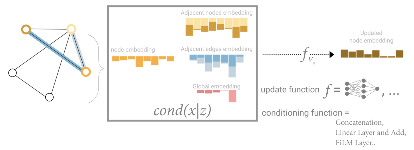
Schematic for conditioning the information of one node based on three other embeddings (adjacent nodes, adjacent edges, global). This step corresponds to the node operations in the Graph Nets Layer.
基于其他三种embeddings (相邻节点、相邻边、全局)来调节一个节点信息的示意图。此步骤对应于图网层中的节点操作。

参考文献

[18] Neural Message Passing for Quantum Chemistry Gilmer, J., Schoenholz, S.S., Riley, P.F., Vinyals, O. and Dahl, G.E., 2017. Proceedings of the 34th International Conference on Machine Learning, Vol 70, pp. 1263--1272. PMLR.

[19] Relational inductive biases, deep learning, and graph networks Battaglia, P.W., Hamrick, J.B., Bapst, V., Sanchez-Gonzalez, A., Zambaldi, V., Malinowski, M., Tacchetti, A., Raposo, D., Santoro, A., Faulkner, R., Gulcehre, C., Song, F., Ballard, A., Gilmer, J., Dahl, G., Vaswani, A., Allen, K., Nash, C., Langston, V., Dyer, C., Heess, N., Wierstra, D., Kohli, P., Botvinick, M., Vinyals, O., Li, Y. and Pascanu, R., 2018.

[20] Deep Sets Zaheer, M., Kottur, S., Ravanbakhsh, S., Poczos, B., Salakhutdinov, R. and Smola, A., 2017.

[21] Molecular graph convolutions: moving beyond fingerprints Kearnes, S., McCloskey, K., Berndl, M., Pande, V. and Riley, P., 2016. J. Comput. Aided Mol. Des., Vol 30(8), pp. 595--608.

< name = "ref22">[22] Feature-wise transformations Dumoulin, V., Perez, E., Schucher, N., Strub, F., Vries, H.d., Courville, A. and Bengio, Y., 2018. Distill, Vol 3(7), pp. e11.